Simulation And Modeling Theory

March 10, 2026

Why Use a Model Instead of the Real System?

Cost: Real-world experiments are expensive. Crashing a real car to test a bumper is far more costly than running a digital crash simulation.
Risk: Experimenting on a live system can cause disasters. A hospital shouldn’t “try out” a new surgery schedule on real patients to see if it works; they should simulate it first.
Feasibility: Often, the system doesn’t exist yet. You can’t test a bridge or a new computer chip until you’ve modeled it to ensure the design is sound.

Different between the actual system and Model of system

Feature	Actual System	Model of System
What it is	The real-life, physical operation.	A mathematical or physical “stand-in.”
Reliability	100% Valid. The results are real.	Questionable. Only as good as the math.
Cost	Very High. Expensive to change.	Low. Cheap to run on a computer.
Risk	High. Could crash or lose customers.	Zero. Failure happens on a screen.
Usage	Used when changes are easy/safe.	Used when systems don’t exist yet.

Here is a simple breakdown of the differences to help you prepare for an exam:

Physical Model vs. Mathematical Model

Feature	Physical Model	Mathematical Model
Form	Tangible / Object	Logical / Equations
Flexibility	Hard to change once built	Easy to change numbers/code
Usage	Engineering & Training	Business & System Analysis
Cost	High (materials/labor)	Low (mostly computer time)

Analytical Solution vs. Simulation

Feature	Analytical Solution	Simulation
Result	Exact (Closed-form)	Estimate (Numerical)
Complexity	Best for simple systems	Best for complex systems
Method	Paper/Pencil or simple math	Computer “exercise” of the model
Certainty	Guaranteed answer	“What if” scenarios

To understand this for an exam, focus on whether the “clock” matters.

Static vs. Dynamic Simulation

Feature	Static Model	Dynamic Model
Time Element	Time is ignored (not a factor).	Time is essential (system evolves).
Visual Analogy	A Snapshot / Photograph.	A Video / Animation.
Key Example	Monte Carlo (Probability) models.	Factory lines, Traffic flow.

For an exam, the difference between these two comes down to one word: Randomness.

Deterministic vs. Stochastic Models

Feature	Deterministic	Stochastic
Randomness	None (Fixed)	Yes (Probabilistic)
Predictability	100% predictable	Variable results
Output Type	Exact Value	Statistical Estimate
Best Example	Mathematical Equations	Queueing (Lines) / Inventory

To understand this for an exam, focus on how the system changes. It isn’t just about what the system is, but how you choose to view it.

Continuous vs. Discrete Simulation

Feature	Discrete	Continuous
Changes	At specific points (Events).	Constantly (Smoothly).
Clock	Jumps from event to event.	Moves continuously.
Math	Logic and “If/Then” events.	Differential equations.
Focus	Individual items/people.	The system as a whole (flow).

What is Discrete-Event Simulation (DES)?

Discrete-event simulation is the modeling of a system as it moves through time. The most important feature is that the state of the system only changes at specific moments.

Example for Exam: A Barber Shop

Event 1: A customer arrives. (The state changes from 0 to 1 person in the shop).

Empty Space: While the barber is cutting hair, nothing “changes” in the model’s data.

Event 2: The haircut ends and the customer leaves. (The state changes from 1 to 0).

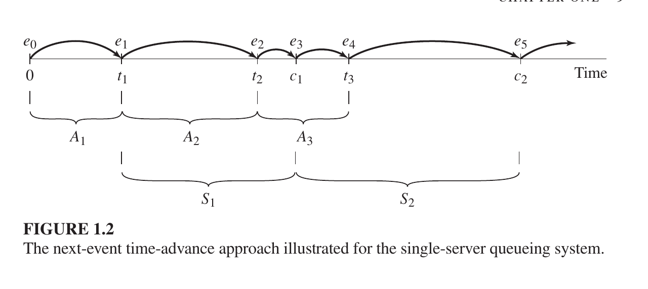
Next-Event Time-Advance (The “Jump” Method)

Instead of watching every empty second, the computer “jumps” directly from one event to the next.

How it works: The clock starts at 0. The computer looks at a list of future events (like a customer arriving or a service finishing) and jumps straight to the time of the very next event.

Why it’s better: It skips over periods where nothing is happening, which saves a lot of computer processing time.

Variable Jumps: Because events happen at random times, the “jumps” are usually unequal (e.g., jumping 2 minutes, then 10 minutes, then 1 minute).

A Simple Example: The Single-Server Queue (oner service provider and one a customer)

Imagine a small coffee shop with one worker. Here is how the simulation clock moves:

b. Start (Time 0): The shop is empty. The computer calculates when the first customer will arrive (let’s say at Minute 5).

c. Event 1 (Arrival): The clock jumps to Minute 5. The customer arrives. Since the worker is free, they start making coffee. The computer calculates the coffee will take 3 minutes to make, so the “Service Completion” event is set for Minute 8.

d. Next Event? The computer checks: Is the next event another arrival or a completion?

e. If a new person arrives at Minute 7, the clock jumps to Minute 7.

f. Since the worker is busy, this new person joins a line (the queue).

g. Event 3 (Completion): The clock jumps to Minute 8. The first customer leaves. The second person in line starts their service.

A system

is defined to be a collection of entities, e.g., people or machines, that act and interact together toward the accomplishment of some logical end.

The application of simulation and Modeling

Factories & Mines: Planning how to build products, layout assembly lines, and move minerals efficiently.
Business & Services: Improving wait times at hospitals, fast-food restaurants, and call centers, or rethinking how a company operates.
Transportation: Designing better flow for airports, subways, and highways to reduce traffic jams.
Tech & Communications: Testing how much data a network can handle or what hardware a new computer needs.
Shipping & Supply Chains: Deciding how much stock to keep in warehouses and the best way to deliver goods.
Military: Testing new weapons and figuring out how to get supplies to troops safely.

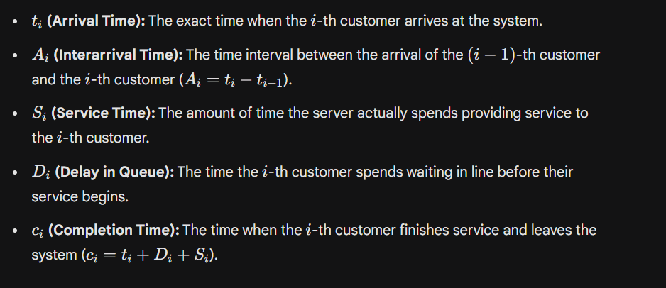
The component of Discrete event simulation

1. System State: A description of the system’s condition at a specific time. For example: How many people are in a bank line, or is the server busy or free?

2. Simulation Clock: A variable that tracks the current time of the simulation.

3. Event List: A list of when future events will occur. For example: “The next customer will arrive at 10:05 AM.”

4. Statistical Counters: Variables used to store information about system performance. For example: Total number of customers who arrived or the average waiting time.

5. Initialization Routine: A subprogram to set all variables at the start of the simulation (Time 0). For example: Setting the clock to 0 and ensuring the line is empty.

6. Timing Routine: A subprogram that determines the next event from the event list and advances the simulation clock to that time.

7. Event Routine: A subprogram that updates the system state when a specific type of event occurs.

The Next-Event Time-Advance Approach

is the standard method used in simulation to move the “clock” forward. Instead of moving second-by-second, the simulation jumps from the time of one event directly to the time of the next scheduled event.

The “Flow of Control”

refers to how the different parts of the simulation program talk to each other.

Single server queue

is the most basic model of simulation and queuing theory. It is a system where there is only one server and people or objects waiting to be served wait in a queue.

The objective of single server queue

we typically want to know three things:

Average Delay in Queue: How long a customer has to wait in line on average.
Time-Average Number in Queue: How many customers are in line on average.
Server Utilization: What percentage of the time is the server (or barber) busy.

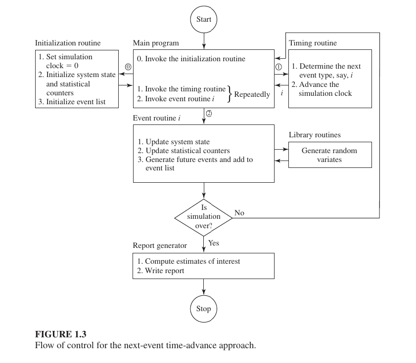
Custormer number chance with respect to time

The Average Number in Queue

is calculated to understand how much congestion a system can handle. It is usually expressed as q.

$$\hat{q}(n) = \frac{\text{Total Area under } Q(t) \text{ curve}}{\text{Total Time } T(n)}$$

Visualizing the Calculation

Imagine your queue length changes like this:

0 to 2 minutes: 0 people ($Area = 2 \times 0 = 0$)
2 to 5 minutes: 1 person ($Area = 3 \times 1 = 3$)
5 to 8 minutes: 2 people ($Area = 3 \times 2 = 6$)

Total Area = $0 + 3 + 6 = 9$ Total Time ($T$) = 8 minutes

Average ($\hat{q}$) = $9 \div 8 = 1.125$ customers.

Server Busy

General Formula for Exams:

$$\hat{u}(n) = \frac{\int_{0}^{T(n)} B(t) dt}{T(n)}$$

Server Utilization or Busy Status ($\hat{u}(n)$)

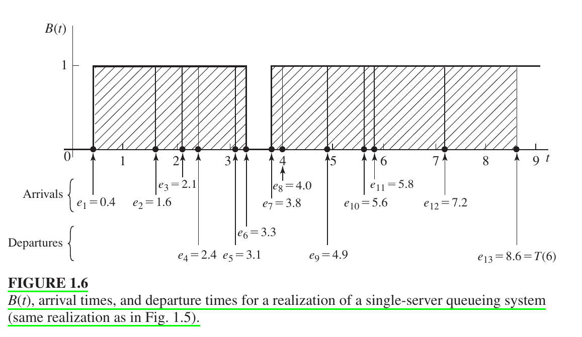
To determine how long the server was working, we use the Busy Function $B(t)$.

If the server is busy, $B(t) = 1$.
If the server is idle (free), $B(t) = 0$.

Calculation:

In the provided figure, the server was busy in two distinct blocks of time:

First Block: From $0.4$ to $3.3$ (Duration = $2.9$)
Second Block: From $3.8$ to $8.6$ (Duration = $4.8$)

Total Busy Time: $2.9 + 4.8 = 7.7$
Total time =8.6
Utilization $\hat{u}(n)$: $$\hat{u}(n) = \frac{7.7}{8.6} \approx 0.90$$

Meaning: This result (0.90) indicates that the server was busy 90% of the time during the simulation.

Inutative problem of single server queue

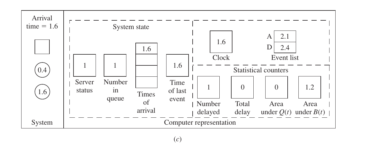
1. System State (Current Status)

Server Status (1): The server is Busy (it is still serving the first customer who arrived at 0.4).
Number in Queue (1): Since the server is busy, the new customer (who just arrived at 1.6) must wait in line.
Times of Arrival [1.6]: The system records that a customer entered the queue at time 1.6. This is needed later to calculate their delay.
Time of Last Event (1.6): The clock has just jumped to 1.6, so the “most recent” event time is updated.

2. Clock and Event List (The Schedule)

Clock (1.6): The simulation clock is now at 1.6.
Event List:
- A (Next Arrival) = 2.1: The system has generated a random number and determined the 3rd customer will arrive at 2.1.
- D (Next Departure) = 2.4: The first customer (who started service at 0.4) is scheduled to finish at 2.4.
- Decision: Since $2.1 < 2.4$, the next event will be another Arrival.

3. Statistical Counters (The Records)

This is where the math happens. Look at how the areas are updated before the state changes:

Number Delayed (1): The first customer already entered service (at time 0.4), so 1 person has “completed” their delay (which was 0).
Area under $B(t)$ (1.2): This is very important.
- Between the last event (0.4) and this event (1.6), the server was Busy.
- Time elapsed = $1.6 - 0.4 = 1.2$.
- Since $B(t) = 1$, the area added is $1 \times 1.2 = 1.2$.
Area under $Q(t)$ (0): Between 0.4 and 1.6, the queue was empty. So, $0 \times 1.2 = 0$. The area remains 0.

$\text{New Area } Q = \text{Old Area } Q + (\text{Number in Queue} \times (T_{now} - T_{old}))$
$\text{New Area } B = \text{Old Area } B + (\text{Server Status} \times (T_{now} - T_{old}))$

An Event Graph

Nodes (Circles): Each node represents a specific Event (such as an Arrival or a Departure).
Arcs (Arrows): The arrows represent the relationship between events, showing how one event schedules another event to occur at a future point in time.is a simplified diagram used to represent the logic of a simulation model.

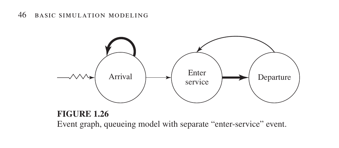
Here is the English translation for the three main events in your Event Graph:

This graph consists of three nodes (circles), each representing a distinct event:

Arrival: Occurs when a new customer enters the system.
Enter Service: Occurs when a customer reaches the server and their service begins.
Departure: Occurs when a customer’s service is completed and they exit the system and check there are any new customer in the queue.

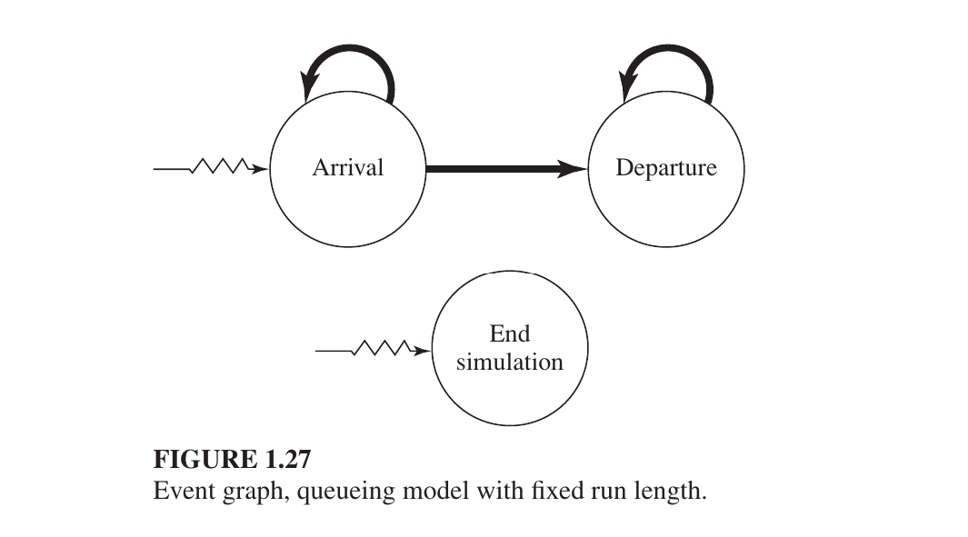
Arrow from Arrival towards itself: This indicates that when a customer arrives, he will also schedule the time when the next customer will arrive. As a result, the process of customer arrival continues.

Arrow from Arrival to Departure: When a customer arrives and sees that the server is empty, his service will start and he will schedule his departure time.

Arrow from Departure towards himself: This is a special logic. If there are more customers waiting in the line, when one leaves, the service of the next customer will start (which in turn schedules his Departure event).

End Simulation (separate part below): This event is not directly related to any of the above. It is an independent event. The time at which the simulation starts (Time 0) is set to a specific time (e.g. 8 hours later). When the clock strikes that time, this event will be triggered and all processes will stop and generate a report.

inventory management sysytem

Key Components of the Graph:

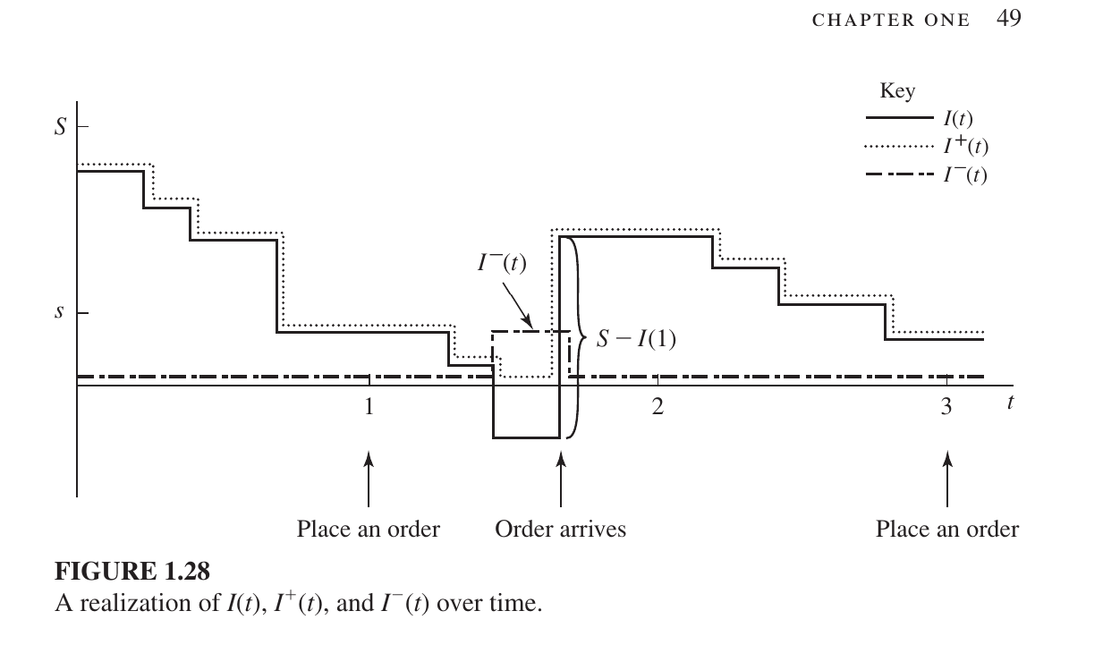
$I(t)$ (Solid Line): This is the actual inventory level. It can be positive (stock available) or negative (backlog/shortage).
$I^{+}(t)$ (Dotted Line): This represents on-hand inventory. It only tracks positive stock; when $I(t)$ goes negative, this line stays at zero.
$I^{-}(t)$ (Dashed Line): This represents the backlog or shortage. When $I(t)$ is negative (meaning customer demand exists but there is no stock), this line moves above zero to show the deficit.
$S$ and $s$:
- $S$ (Maximum Level): The target maximum stock level.
- $s$ (Reorder Point): The threshold level; when inventory falls below this point, a new order is triggered.

Step-by-Step Breakdown:

Decreasing Steps: The downward steps indicate customer arrivals and product sales, which gradually deplete the stock.
Place an Order: When the inventory level $I(t)$ drops below the reorder point $s$, an order is placed (seen at the 1-month mark).
Order Arrives: After a certain delay (lead time), the order arrives. The graph shoots up vertically as the new stock is added.
Backlog/Shortage: In the middle of the graph, $I(t)$ drops below zero, indicating a shortage. When the new order ($S - I(1)$) arrives, it first satisfies the backlog, and the remainder becomes the new positive inventory.

These images show the formulas and simulation parameters for evaluating the Inventory System. Here is a breakdown of the mathematical formulas and the simulation setup:

1. Time-Average Calculations

To calculate the total cost, the simulation finds the time-average of items held in inventory and items in backlog over $n$ months.

Average Holding (Items on hand): $$\bar{I}^+ = \frac{\int_{0}^{n} I^+(t) , dt}{n}$$ The average holding cost per month is then calculated as $h\bar{I}^+$.
Average Backlog (Shortage): $$\bar{I}^- = \frac{\int_{0}^{n} I^-(t) , dt}{n}$$ The average backlog cost per month is $\pi\bar{I}^-$ (where $\pi = $5$ per item per month).

3. Inventory Policies to Compare

The simulation tests nine different combinations of $s$ (reorder point) and $S$ (target level):

$s$	20	20	20	20	40	40	40	60	60
$S$	40	60	80	100	60	80	100	80	100

The Scenario (2 Months)

Month 1 (Good Days): You have 10 bats in your shop. No one bought them all, so for the whole month, you just kept those 10 bats on the shelf.
Month 2 (Bad Days): You ran out of bats! 5 customers came and asked for bats, but you couldn’t give them any. They are waiting for you to get new stock. This is your Backlog.

1. The Holding Cost (ভাড়া বা রক্ষণাবেক্ষণ খরচ)

The landlord charges you $1 per month for every bat you keep in the shop.

In Month 1, you kept 10 bats. Cost = $10$.
In Month 2, you kept 0 bats. Cost = $0$.
Total cost for 2 months = $10 + 0 = $10$.

Now, to find the Average Monthly Cost, we divide by 2 months:

$10 \div 2 = $5$ per month. (This is your average holding cost).

2. The Backlog Cost (কাস্টমারকে বসিয়ে রাখার জরিমানা)

Because customers had to wait in Month 2, it hurts your reputation. Let’s say this “bad reputation cost” is $5 per month for every customer waiting.

In Month 1, 0 customers were waiting. Cost = $0$.
In Month 2, 5 customers were waiting. Cost = $5 \text{ customers} \times $5 = $25$.
Total cost for 2 months = $0 + 25 = $25$.

Now, to find the Average Monthly Backlog Cost, we divide by 2 months:

$25 \div 2 = $12.5$ per month.

3. Total Average Cost

Now, simply add the two averages together to see how much money you are losing/spending on average every month to run this shop:

Average Holding: $5
Average Backlog: $12.5
Total: $5 + 12.5 = \mathbf{$17.5}$

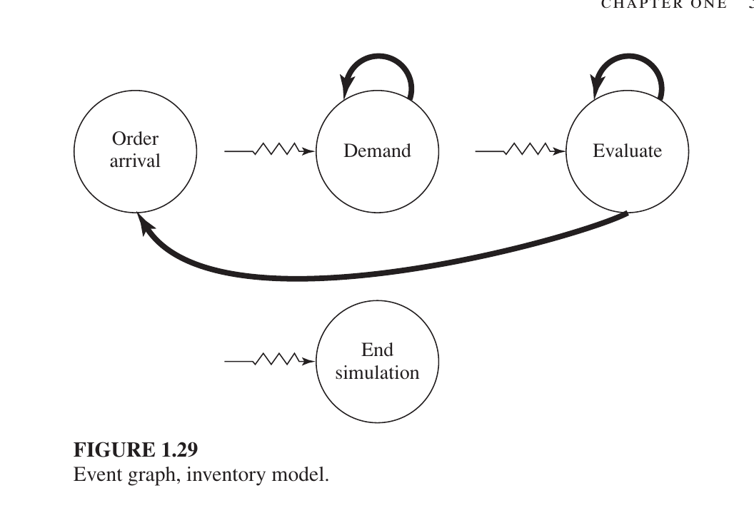
The Events (The Circles)

Demand: A customer wants to buy something. This circle has a loop on top, meaning one customer’s arrival schedules the next customer’s arrival.

Evaluate: The system checks the stock level (usually at the start of each month) to see if it’s time to order more. The loop on top means it schedules itself to check again next month.

Order Arrival: This happens when the products you ordered finally show up at the warehouse.

End Simulation: The “stop” button that closes the program after the set time (e.g., 120 months) is up.

What is Parallel Simulation?

Usually a simulation runs sequentially on a computer. But if the model is very large (eg: a network with thousands of nodes or a huge battle model), it takes a long time to run. In parallel simulation, the model is divided into several parts and run on separate processors. Its purpose is to reduce the simulation completion time by dividing the work.

what is sound simulation study

refers to a disciplined, systematic process for designing and analyzing complex systems using simulation. It ensures that the results are not just “computer output,” but are statistically valid, logically verified, and practically useful for decision-making.

The 10 Essential Steps of a Sound Simulation Study

To ensure a study is “sound” (reliable), researchers typically follow these steps:

Problem Formulation: Clearly define the goals of the study. What specific questions are you trying to answer? (e.g., “How many tellers do we need to keep wait times under 5 minutes?”)
Data Collection & Model Specification: Gather real-world data (like arrival rates or service times) and define the logic of how the system works.
Conceptual Model Validation: Before coding, check with subject matter experts to ensure your logical “blueprint” is correct.
Programming (Translation): Convert the logic into a computer program using languages like Python, C++, or specialized tools like Arena or AnyLogic.
Verification: This is “debugging.” Does the code do what the logic intended?
Validation (The “Realism” Check): Compare the simulation output to data from the actual system. If the simulation says a bank serves 100 people an hour, but the real bank only serves 50, the model is not valid.

7. Experimental Design: Decide on the “what-ifs.” Which parameters (like the number of machines or worker shifts) will you change to see the impact? 8. Production Runs: Run the simulation enough times to get a significant sample size. 9. Output Analysis: Use statistical methods (like confidence intervals) to interpret the results. Since simulations involve randomness, you cannot rely on just one run. 10. Documentation and Implementation: Present the findings and use them to make real-world changes.

Why is this process necessary?

Without these steps, a simulation might suffer from “GIGO” (Garbage In, Garbage Out). If your input data is wrong or your model isn’t validated, you might make a multi-million dollar business decision based on a faulty computer program.

1. Advantages of Simulation

Simulation is a widely popular method for studying complex systems because:

Analyzing Complex Systems: Many real-world systems are too complex to be solved with simple math. Simulation is often the only way to investigate them.
Future Prediction: It allows you to estimate how a system will perform under projected future conditions.
Comparing Alternatives: You can compare different system designs or policies to see which one best meets your requirements.
Total Control: You have much better control over experimental conditions (like speed or input) than you would in a real-world test.
Time Compression/Expansion: You can simulate years of data in minutes (Time Compression) or slow down a very fast process to see exactly what is happening (Time Expansion).

2. Disadvantages of Simulation

Estimates, Not Exact Answers: Results are just estimates of a model’s true characteristics. You often need to run the simulation many times (multiple replications) to get a reliable average.
High Cost and Time: Developing a high-quality, valid simulation model can be expensive and take a long time.
False Confidence: People often place too much trust in results because of impressive animations or large amounts of data. If the model is wrong, the results are useless.

3. Common Pitfalls (Mistakes to Avoid)

Many simulation projects fail because of these common errors:

Undefined Objectives: Starting without a clear goal of what you want to solve.
Inappropriate Level of Detail: Making the model way too complex (wasting time) or way too simple (losing accuracy).
The “Programming” Trap: Treating the study as just a coding exercise while ignoring the necessary statistics and methodology.
Bad Data: Running a simulation using incorrect or insufficient real-world information.
Ignoring Randomness: Failing to correctly account for the unpredictable parts of the system.
Single Replication: Running the simulation only one time and treating that single result as the absolute “truth.”

Comparison Between Single-Server and Queueing system (Multi-Server Systems)

Feature	Single-Server ($M/M/1$)	Multi-Server ($M/M/s$)
Number of Servers	One ($s = 1$)	Multiple ($s > 1$)
Service Capacity	Limited; only one customer at a time. $\rho = \frac{\lambda}{ \omega}$	Much higher; up to $s$ customers at once. $\rho = \frac{\lambda}{s\omega}$
Waiting Time	Generally longer.	Generally shorter due to load sharing.
System Risk	If the server fails, the entire system stops.	If one server fails, others remain operational.

Random Variable

A Random Variable is a function or rule that assigns a numerical value to each outcome in a sample space. It essentially maps experimental results to real numbers. It is primarily of two types:

Discrete Random Variable: These take on values that can be counted (e.g., the number of family members, the outcome of rolling a die).
Continuous Random Variable: These can take on any real value within a certain range (e.g., temperature, height, time).

Probability Functions

These functions are used to understand how a variable is distributed:

A. Probability Mass Function (PMF) - $p(x)$

The PMF is used for Discrete random variables. It indicates the probability of the variable being exactly equal to a specific value $x$.

Condition: $\sum p(x_i) = 1$

Example: Suppose you roll a fair die. The possible outcomes ($x$) are 1, 2, 3, 4, 5, or 6. Since each number has an equal chance of appearing, the PMF is:

$p(1) = 1/6$
$p(2) = 1/6$
…
$p(6) = 1/6$

If you sum them all up: $1/6 + 1/6 + 1/6 + 1/6 + 1/6 + 1/6 = 1$.

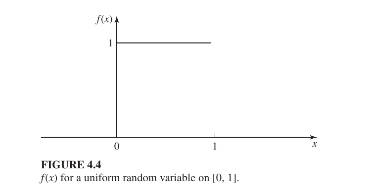
B. Probability Density Function (PDF) - $f(x)$

The Probability Density Function (PDF) describes the behavior of a Continuous Random Variable. Unlike discrete variables, continuous variables can take any value within a range (like time, temperature, or height).

1. Key Properties

A function $f(x)$ is considered a PDF if it meets these conditions:

Non-negative: The value is always zero or positive, $f(x) \geq 0$.
Total Area is 1: The total area under the curve must equal 1: $$\int_{-\infty}^{\infty} f(x) dx = 1$$
Point Probability is 0: For a continuous variable, the probability of an exact single point is always zero, $P(X = a) = 0$. We always calculate probability over an interval or range, such as $P(a \leq X \leq b)$.

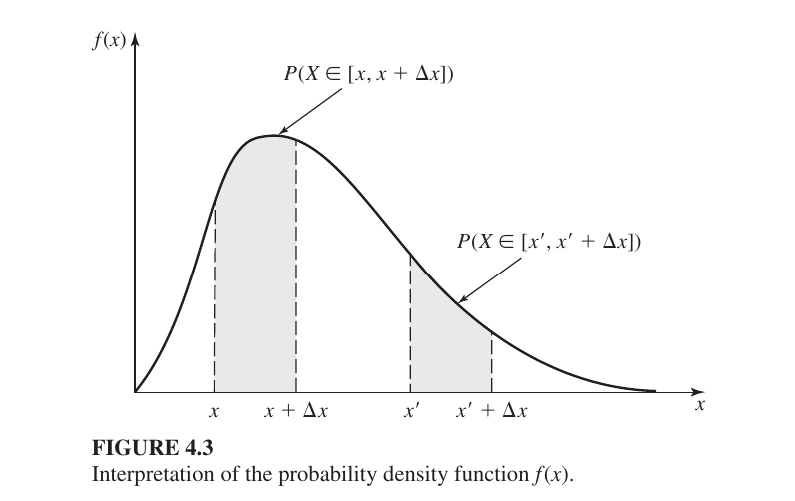
First Interval: $[x, x + \Delta x]$This represents the probability that $X$ lies between $x$ and $x + \Delta x$. If this interval contains a “step” (a jump in the graph), it means there is a non-zero probability of $X$ taking a value in that range.

Second Interval: $[x’, x’ + \Delta x]$This is another interval of the same width ($\Delta x$) but at a different location ($x’$).

2. Practical Example: Battery Life

Suppose a company makes batteries that last anywhere from 0 to 5 years. Let $X$ be the battery life. This is a Continuous Uniform Distribution, where the PDF is:

$$f(x) = \begin{cases} \frac{1}{5} & 0 \leq x \leq 5 \ 0 & \text{otherwise} \end{cases}$$

Why is the value $1/5$? Since the total area must be 1 and the width of our range is 5 (from 0 to 5), the height must be $1/5$ because: $$\text{Area} = \text{Width} \times \text{Height} = 5 \times \frac{1}{5} = 1$$

Calculating Probability: To find the probability that a battery lasts between 2 and 4 years, we calculate the area between 2 and 4: $$P(2 \leq X \leq 4) = \int_{2}^{4} \frac{1}{5} dx = \left[ \frac{x}{5} \right]_{2}^{4} = \frac{4}{5} - \frac{2}{5} = \frac{2}{5} = 0.4 \text{ or } 40%$$

3. PMF vs. PDF: The Main Difference

Feature	PMF (Probability Mass Function)	PDF (Probability Density Function)
Data Type	Discrete (Countable: 1, 2, 3…)	Continuous (Measurable: 1.5, 2.7…)
Exact Point	$P(X=x)$ has a specific value.	$P(X=x)$ is always 0.
How to find Probability	Look at the specific point or sum them.	Calculate the Area under the curve.
Calculation	Uses Summation ($\sum$)	Uses Integration ($\int$)

C. Cumulative Distribution Function (CDF) - $F(x)$

The Cumulative Distribution Function (CDF) represents the accumulated probability up to a certain point. In simple terms, it tells us the total probability that the random variable $X$ will take a value less than or equal to $x$. $$F(x) = P(X \leq x)$$

Three criteria for CDF

1. The Value is Always Between 0 and 1

Since $F(x)$ represents a probability ($P(X \leq x)$), its value can never be negative and can never exceed 100%. $$0 \leq F(x) \leq 1$$

2. It Never Goes Down (Non-decreasing)

As you move from left to right on the x-axis, the accumulated probability either increases or stays the same. It can never drop because you are always adding more (or zero) probability as you include more possible values of $x$.

If $x_1 < x_2$, then $F(x_1) \leq F(x_2)$

3. The Boundaries (Starts at 0, Ends at 1)

At the far left ($-\infty$): The probability of the variable being “less than negative infinity” is 0.
At the far right ($+\infty$): The probability of the variable being “less than positive infinity” is 1 (because it must eventually take some value).

$$\lim_{x \to -\infty} F(x) = 0 \quad \text{and} \quad \lim_{x \to \infty} F(x) = 1$$

Discrete Example: Rolling a Die

Suppose you roll a fair die. The outcomes are $1, 2, 3, 4, 5, 6$, each with a probability ($p(x)$) of $1/6$. The CDF values are calculated by adding up the probabilities:

$F(1)$: Probability of 1 or less = $1/6 \approx 0.16$
$F(2)$: Probability of 2 or less = $p(1) + p(2) = 2/6 \approx 0.33$
$F(3)$: Probability of 3 or less = $p(1) + p(2) + p(3) = 3/6 = 0.50$
…
$F(6)$: Probability of 6 or less = $6/6 = 1.00$

Continuous Example: Bus Arrival Time

Suppose a bus arrives any time between 0 and 5 minutes. The PDF was $f(x) = 1/5$. The CDF is the total area under the PDF curve from the start up to point $x$: $$F(x) = \int_{0}^{x} f(y) dy = \int_{0}^{x} \frac{1}{5} dy = \frac{x}{5}$$

$F(0)$: Probability of arrival at 0 mins = $0/5 = 0$
$F(2.5)$: Probability of arrival within 2.5 mins = $2.5/5 = 0.5$ (50% chance)
$F(5)$: Probability of arrival within 5 mins = $5/5 = 1$ (100% certain)

Graph for CDF

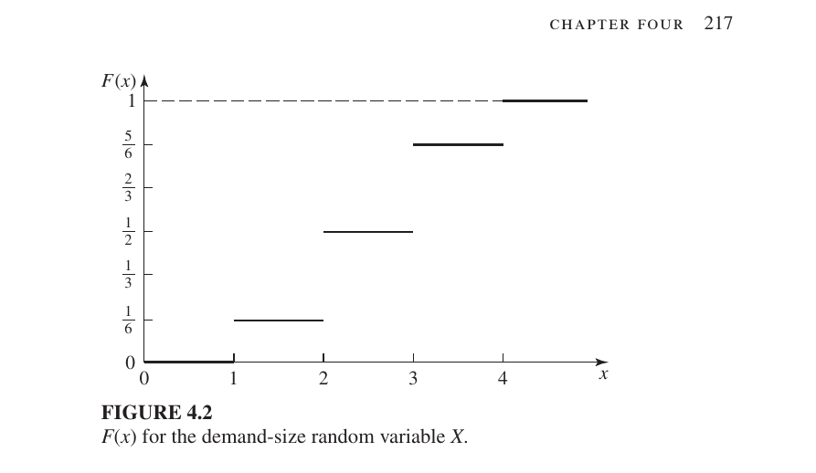
Understanding the CDF Values The CDF represents the probability that the random variable $X$ will take a value less than or equal to $x$, i.e., $F(x) = P(X \le x)$. From the step function in the image, we can define $F(x)$ as follows:

For $x < 1$: $F(x) = 0$
For $1 \le x < 2$: $F(x) = 1/6$
For $2 \le x < 3$: $F(x) = 1/2$
For $3 \le x < 4$: $F(x) = 5/6$
For $x \ge 4$: $F(x) = 1$

Example 4.7

What happens if $x < 0$ or $x > 1$?

The text asks: “What is $F(x)$ if $x < 0$ or if $x > 1$?”

If $x < 0$: $F(x) = 0$. This is because no probability has accumulated before the starting point of 0.
If $x > 1$: $F(x) = 1$. This is because 100% of the probability has already been accounted for by the time $x$ reaches 1; it cannot increase further.

The Complete CDF Function

Combining all conditions, the full $F(x)$ function is defined as: $$F(x) = \begin{cases} 0 & \text{for } x < 0 \ x & \text{for } 0 \le x \le 1 \ 1 & \text{for } x > 1 \end{cases}$$ Visually, the CDF graph starts at $(0,0)$, climbs as a straight diagonal line to $(1,1)$, and then remains horizontal at the value of 1.

Discussion for PMF & PDF & CDF

While PMF or PDF describes the probability at a specific point or density, the CDF describes the “running total” of probability. In simulation (like the inventory models in your text), the CDF is crucial because it allows computers to map a random number (between 0 and 1) to a specific real-world outcome.

Example 4.10

This analysis explains why the two events—drawing an Ace and drawing a King from a deck without replacement—are not independent. It compares the Joint Probability to the product of the Marginal Probabilities.

Joint Probability: $p(1, 1)$

The notation $p(1, 1)$ represents the probability of getting exactly 1 Ace and 1 King when drawing two cards from a deck of 52.

$$p(1, 1) = 2 \left( \frac{4}{52} \right) \left( \frac{4}{51} \right)$$

Mathematical Analysis of Marginal Probabilities

Let $X$ be the number of Aces and $Y$ be the number of Kings. To check for independence, we calculate the product of their marginal probabilities.

The marginal probability of getting exactly one Ace ($p_X(1)$) is: $$p_X(1) = 2 \cdot \left( \frac{4}{52} \right) \cdot \left( \frac{48}{51} \right)$$ (One Ace and one “non-Ace” card)

Similarly, for one King ($p_Y(1)$): $$p_Y(1) = 2 \cdot \left( \frac{4}{52} \right) \cdot \left( \frac{48}{51} \right)$$

Now, multiplying them together: $$p_X(1) \times p_Y(1) = \left[ 2 \cdot \frac{4}{52} \cdot \frac{48}{51} \right] \times \left[ 2 \cdot \frac{4}{52} \cdot \frac{48}{51} \right]$$ $$= 4 \cdot \left( \frac{4}{52} \right)^2 \cdot \left( \frac{48}{51} \right)^2$$

3. The Core Difference (Conclusion)

To prove independence, the following condition must be met: $p(x, y) = p_X(x) \times p_Y(y)$.

However, as we can see:

Actual Joint Probability: $p(1, 1) = 2 \cdot \frac{4}{52} \cdot \frac{4}{51}$
Product of Marginals: $p_X(1) \times p_Y(1) = 4 \cdot (\frac{4}{52})^2 \cdot (\frac{48}{51})^2$

Since $p(1, 1) \neq p_X(1) \times p_Y(1)$, the events are not dependent.

Example 3.15

This description explains the concept of Variance ($\sigma^2$), the method for calculating it, and its visual representation on a graph. Variance measures how much a distribution “spreads out” from its mean ($\mu$).

Here is the explanation in English:

Mathematical Calculation

In this example, the variance is calculated for a discrete random variable $X$.

Step 1 (Find $E(X^2)$): Multiply the square of each value ($x^2$) by its corresponding probability ($P(X=x)$) and sum them up. $$E(X^2) = 1^2\left(\frac{1}{6}\right) + 2^2\left(\frac{1}{3}\right) + 3^2\left(\frac{1}{3}\right) + 4^2\left(\frac{1}{6}\right) = \frac{43}{6}$$
Step 2 (Variance Formula): The standard formula for variance is $\text{Var}(X) = E(X^2) - \mu^2$. Given the mean $\mu = 5/2$: $$\text{Var}(X) = \frac{43}{6} - \left(\frac{5}{2}\right)^2 = \frac{43}{6} - \frac{25}{4} = \frac{11}{12}$$
Variance tells us the degree of “spread” in the data.
Higher Variance: Indicates higher uncertainty or greater deviation from the average.
Lower Variance: Indicates more consistency, with data staying close to the average.

Covariance

measures the joint variability of two random variables, indicating how they move together

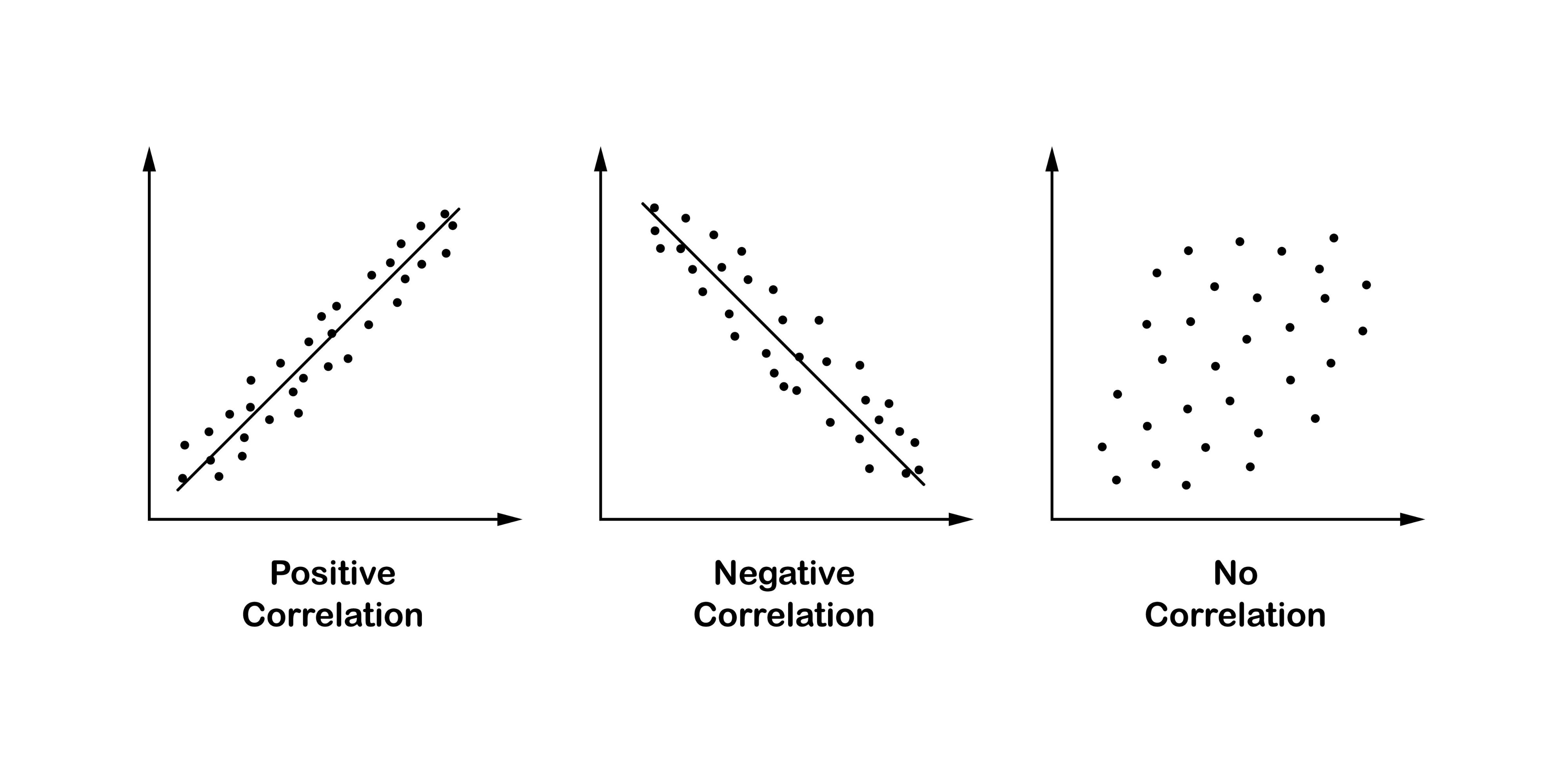
Correlation: The Strength and Scale

Correlation (specifically the Correlation Coefficient) tells us exactly how strong that relationship is on a standardized scale (usually from -1 to +1).

Values and Their Meanings

The value of the correlation coefficient always ranges from $-1$ to $+1$.

$+1$ (Perfect Positive Relationship): As one variable increases, the other variable increases in a perfectly predictable, linear fashion. On a graph, all data points would fall exactly on a straight line pointing upward.
$-1$ (Perfect Negative Relationship): As one variable increases, the other variable decreases in a perfectly predictable, linear fashion. On a graph, all data points would fall exactly on a straight line pointing downward.
$0$ (No Linear Relationship): There is no straight-line relationship between the two variables. Changes in one variable do not predict changes in the other in a linear way.

Deterministic Process: The Predictable Clockwork

A deterministic process is one where the future state is entirely determined by its current state and a fixed rule. There is no randomness involved; if you know the starting point and the formula, you can predict the outcome with 100% certainty.

** Example: A Bank Account with Fixed Interest** Imagine you deposit $100 into an account that pays exactly 5% interest every year.
- Year 1: You have $105.
- Year 2: You have $110.25.
- Year 10: You can calculate exactly how much you will have down to the last cent. The “system” evolves over time according to a fixed rule: $Future Value = Present Value \times (1 + r)^t$.

Stochastic Process: The Unpredictable Journey

is a mathematical collection of random variables that represents the evolution of a system, value, or signal over time, acting as a random alternative to deterministic processes.

This is an excellent real-world example of a stochastic process. Here is the explanation in English:

Stock Market Prices as a Stochastic Process

In the stock market, the price of a share—let’s call it $S(t)$—changes over time ($t$). This movement is considered a stochastic process because it involves inherent randomness and uncertainty at every step.

The Scenario: Suppose a share is priced at 1,000 BDT today.
The Uncertainty: By tomorrow, the price could drop to 950 BDT or rise to 1,050 BDT.
The Random Element: These fluctuations are driven by unpredictable factors such as market sentiment, global news, or economic shifts. Because the exact future price cannot be determined by a fixed formula, we describe it using probabilities and statistical models.

Why it is Stochastic (Random) vs. Deterministic (Fixed)

Deterministic: If the price increased by exactly 5 BDT every single day without fail, it would be deterministic. You could calculate the price 100 days from now with 100% accuracy.
Stochastic: In reality, even if the “trend” is upward, the day-to-day changes are random. We can estimate the expected value, but we can never be certain of the exact outcome.

Covariance-Stationarity (often called Weak Stationarity)

describes a state where the core statistical properties of a time-series dataset do not change over time. In simple terms, whether you look at data from last year or next year, its fundamental “behavior” or “pattern” remains consistent.

There are the three essential conditions

1. Constant Mean ($\mu$)

The average value of the data must remain constant over time. It should not show a long-term upward trend (growth) or downward trend.

Mathematical Rule: $E[X_i] = \mu$ for all $i$.
Example: If a room’s AC is set to 25°C, the temperature might fluctuate slightly (e.g., 24.8°C to 25.2°C), but the average remains 25°C whether you measure it in the morning or at night.

2. Constant Variance ($\sigma^2$)

The degree of fluctuation or “volatility” in the data must stay roughly the same. The data should not be very calm at one point and extremely volatile at another.

Mathematical Rule: $\text{Var}(X_i) = \sigma^2 < \infty$ for all $i$.
Example: If a stock price fluctuates by $1-$2 every day, its variance is stable. However, if it suddenly starts jumping by $50 or dropping by $100, the variance is no longer constant.

3. Constant Autocovariance

The relationship (covariance) between two data points depends only on the time gap (lag) between them, not on the specific point in time they were measured.

Mathematical Rule: $\text{Cov}(X_i, X_{i+j}) = C_j$ (where $j$ is the lag).
Simple Explanation: The relationship between “today” and “tomorrow” (a 1-day lag) must be the same as the relationship between “data 10 days from now” and “data 11 days from now.” As long as the time difference ($j$) is the same, the correlation remains the same.

Real-World Comparison

Stationary Example: A Climate-Controlled Room

Imagine a room where the temperature is strictly regulated.

The mean is always 25°C.
The fluctuations are always within $\pm$0.2 degrees.
The pattern of how the temperature drops after the compressor turns off is the same every time.
Verdict: This is a Covariance-Stationary process.

Non-Stationary Example: Child Growth or Stock Markets

Child’s Height: A child’s height only increases over time. Because the mean is constantly changing (growing), it is not stationary.
Stock Market: Prices often have “volatility clusters” where the market is calm for weeks and then crashes or spikes violently. Because the variance is not stable, it is not stationary.

Example 4.23

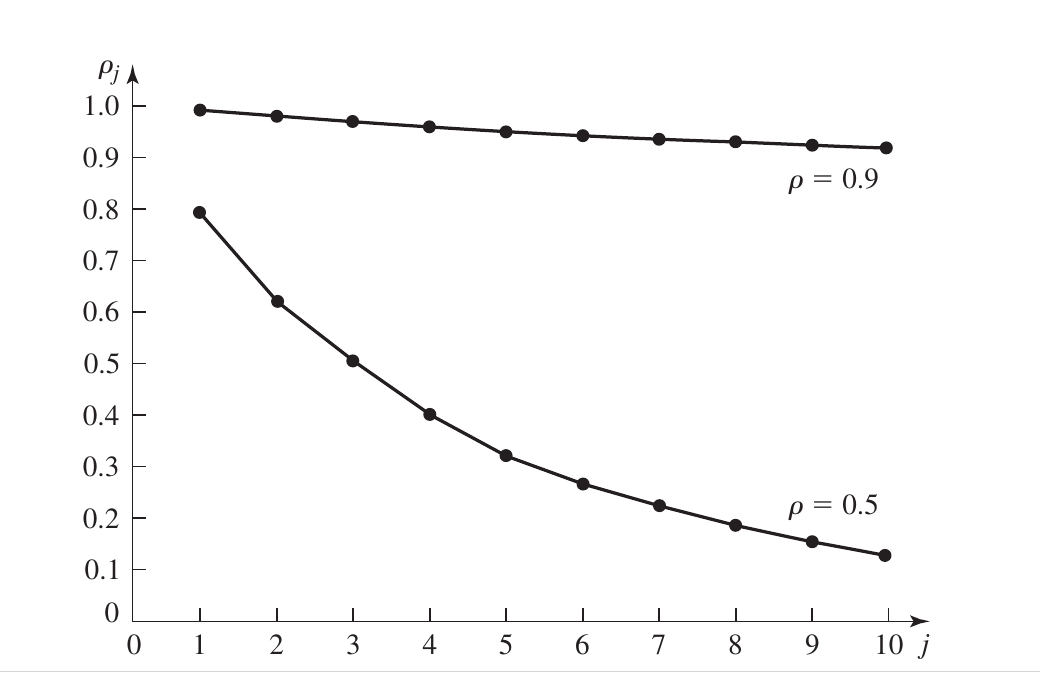
1. Core Components of the Graph

X-axis ($j$ - The Lag): This represents the distance between customers in the queue. For example, a lag of $j=1$ compares a customer with the person immediately behind them, while $j=10$ compares them with the 10th person after them.
Y-axis ($\rho_j$ - Correlation): This measures the strength of the relationship between their waiting times (ranging from 0 to 1). A higher value means their waiting times are very similar.

2. The Impact of Traffic Intensity ($\rho$)

The graph shows two distinct curves representing different levels of system congestion:

High Congestion ($\rho = 0.9$): When the system is very busy (90% utilization), the correlation stays high for a long time and decreases very slowly. This means that if one customer experiences a long delay, it is highly likely that many subsequent customers will also face long delays. This is known as Long-range dependence.
Moderate Congestion ($\rho = 0.5$): When the system is less busy (50% utilization), the correlation drops sharply as the lag increases. The “memory” of the system is short; a delay for one customer doesn’t have a lasting impact on those far behind them in the line.

This part of statistics focuses on Estimation, which is the process of making educated guesses about a large population based on a smaller subset of data.

Here is the explanation in English:

1. Sample Mean ($\bar{X}(n)$): “Finding the Average”

Imagine you want to find the average height of everyone in a country. Measuring millions of people is impossible, so you randomly select 100 people. The average height of these 100 people is called the Sample Mean.

Formula: $\bar{X}(n) = \frac{\sum_{i=1}^{n} X_i}{n}$ (The sum of all heights divided by the number of people).
Property: It is an Unbiased Estimator of the true population mean ($\mu$). This means if you repeat this process many times, the average of all your sample means will eventually equal the true average of the entire population.

2. Sample Variance ($S^2(n)$): “Measuring the Spread”

While measuring heights, you notice some people are 5'2" and others are 6'0". This variation or “spread” in the data is the Variance.

Bessel’s Correction ($n-1$): In the formula for sample variance, we divide by $n-1$ instead of $n$. This adjustment is made to correct the bias in estimating a population’s variance from a sample, ensuring our estimate isn’t too low.

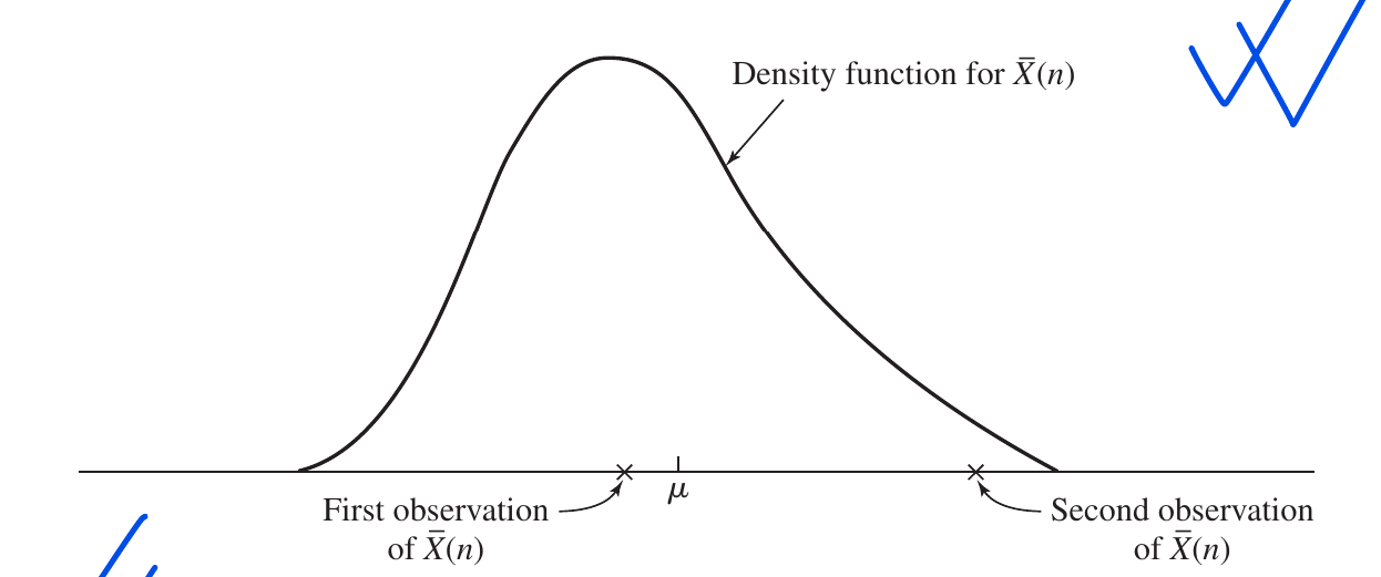
3. Graphical Interpretation (Figure 4.12)

Graphs in this context usually illustrate the Precision and Accuracy of an estimate:

Near the Mean ($\mu$): An observation close to the center indicates a very accurate estimate.
Far from the Mean: An observation far from the center indicates a high margin of error for that specific sample.

Since we never know exactly how close a single sample is to the true mean, we use a Confidence Interval.

A Real-World Example: Biscuit Package Weight

A factory produces biscuit packets labeled “100g.” However, due to machine variations, some packets are 99g and others are 101g.

Sample Mean: You pick 10 packets and find their average weight is 100.5g. This is your $\bar{X}(n)$.
Sample Variance: You calculate how much the weights differ from each other using $S^2(n)$.
Confidence Interval: Based on your data, you can say, “I am 95% confident that the true average weight of all packets produced by this factory is between 100g and 101g.”

Variance of the Sample Mean,

denoted as $\text{Var}[\bar{X}(n)]$. It essentially measures the reliability or the “risk” associated with using a sample average to estimate the true population average.

1. The Mathematical Formula

The variance of the sample mean is derived as: $$\text{Var}[\bar{X}(n)] = \frac{\sigma^2}{n}$$

Where:

$\sigma^2$ is the Population Variance (how much the entire population varies).
$n$ is the Sample Size (how many data points you collected).

Standard Normal Random Variable

($\Phi(z)$)The theorem defines a specific type of normal distribution called the Standard Normal Distribution

Mean ($\mu$) = 0

Variance ($\sigma^2$) = 1

The Integral Formula: $\Phi(z) = \frac{1}{\sqrt{2\pi}} \int_{-\infty}^{z} e^{-y^2/2} dy$

This formula calculates the Cumulative Probability (the area under the bell curve) from negative infinity up to a specific point $z$.

The Central Limit Theorem (CLT)

The CLT is often considered the most important theorem in statistics. it states that regardless of the shape of the original population distribution (even if it is skewed or weird), the distribution of the sample means will approach a Normal Distribution (bell curve) as the sample size ($n$) becomes larger.

The formula shown in your text is: $$Z_n = \frac{\bar{X}(n) - \mu}{\sqrt{\sigma^2/n}}$$ As $n \to \infty$, this $Z_n$ follows a Standard Normal Distribution (Mean = 0, Variance = 1). This allows us to use $Z$-tables to calculate probabilities.

Why use a Confidence Interval?

A single sample mean ($\bar{X}$) is just a “point estimate”—it is almost never exactly equal to the true population mean ($\mu$). Instead of giving a single number, we provide a range (an interval) where we are reasonably sure the true mean lies.

Real-world Example: Saying “The average height is 5'6"” is risky. Saying “I am 95% confident the average height is between 5'4" and 5'8"” is much more scientifically sound.

The Mathematical Formula

$$\bar{X}(n) \pm z_{1-\alpha/2} \sqrt{\frac{S^2(n)}{n}}$$

$\bar{X}(n)$: The sample mean (your starting point).
$z_{1-\alpha/2}$: The critical value from the $Z$-table. For a 95% confidence level, this value is 1.96.
$\sqrt{S^2(n)/n}$: This is the Standard Error (SE). It measures how much the sample mean is expected to vary from the true population mean.

Hypothesis Testing

is a statistical method used to determine whether a specific claim or assumption about a population is supported by sample data.

Null Hypothesis ($H_0$): This is the “Innocent” plea. It represents the status quo, 2. assuming there is no effect, no change, or no difference.
Alternative Hypothesis ($H_1$ or $H_a$): This is the “Prosecution’s” claim. It represents the new theory or the change we are trying to prove.

1. The Mathematical Condition

The rule is expressed as follows:

Reject $H_0$ if: $|t_n| > t_{n-1, 1-\alpha/2}$
Fail to Reject $H_0$ if: $|t_n| \le t_{n-1, 1-\alpha/2}$

Strong Law of Large Numbers (SLLN)?

the SLLN states that as you repeat an experiment and increase your sample size ($n$), the sample mean ($\bar{X}(n)$) will converge to the true population mean ($\mu$) with absolute certainty (probability 1).

Mathematical Expression: $$\bar{X}(n) \to \mu \text{ with probability 1 as } n \to \infty$$

This means that the more data you collect, the closer you get to the “truth,” and the probability of your average being significantly wrong drops to zero.

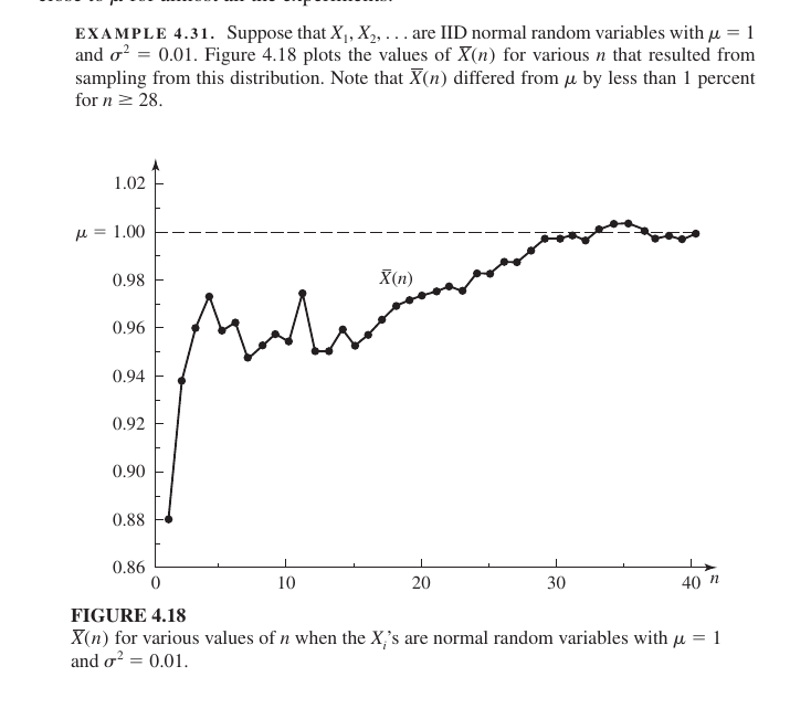
Graphical Interpretatio

The graph shows how the sample mean stabilizes as the number of observations increases:

At the start ($n < 10$): The graph fluctuates wildly. With very little data, the average is highly sensitive to random outliers, leading to high error.
Moving forward ($n = 20$): The fluctuations become smaller as the line approaches the dotted line representing the true mean ($\mu = 1.00$).
The End ($n > 28$): The text notes that by the time $n \ge 28$, the sample mean stays within 1% of the true mean. The graph flattens out and runs almost perfectly parallel to the true mean.

Real-World Example: Coin Tossing

Imagine the probability of getting “Heads” is $0.5$ (50%).

If you toss the coin only 10 times, you might get 7 Heads (an average of $0.7$). This is far from the true average of $0.5$.
If you toss it 1,000 times, you might get 503 Heads (an average of $0.503$).
If you could toss it infinitely, the SLLN guarantees the average would become exactly $0.5$.

the steps involved in a successful Simulation Study:

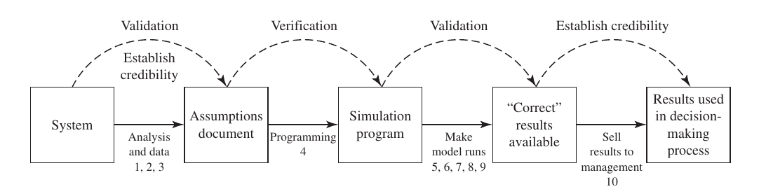
From System to Assumptions Document

First, the real-world System is studied. Logic and data are collected to create an Assumptions Document.

Validation: At this stage, you check if the rules and logic of the system have been correctly recorded in the document.

Programming (Assumptions Document to Simulation Program)

The recorded rules are translated into computer code to create a Simulation Program.

Verification: This is the debugging stage. You ensure the code correctly represents the logic and that the program runs without errors.

Simulation Runs and Results (Program to “Correct” Results)

The program is executed to produce output data or results.

Validation (Second Stage): You compare the simulation results with the behavior of the real system. If they match, the results are considered “Correct.”

Presenting to Management (Selling results)

The final results are presented to the decision-makers or management.

Establish Credibility: This is about trust. If the manager or client believes the model is reliable, the project is considered credible. This is easier if they were involved from the start.

Decision-Making Process

Finally, the credible simulation results are used to make actual changes or new mathematical decisions for the real-world system.

Verification: Was the model built right? (Checking the code).
Validation: Was the right model built? (Comparing with reality).
Credibility: Is the model trusted? (Gaining manager’s confidence).

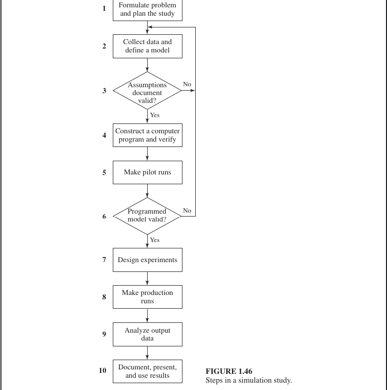
10 steps of a complete simulation study

1. Formulate the Problem

Define the objectives of the simulation. What specific questions are we trying to answer, and what is the ultimate goal of the study? This acts as the foundation for the entire project.

2. Collect Data and Design a Conceptual Model

Gather necessary data from the real-world system (e.g., arrival times, processing speeds). Then, create a “conceptual model” or an Assumptions Document that describes how the system works logically.

3. Validate the Conceptual Model

Before coding, verify the logic with system experts. Does the Assumptions Document accurately reflect the real system? This ensures you aren’t building a model based on wrong ideas.

4. Program the Model

Translate the conceptual model into a computer program using simulation software (like Arena, AnyLogic, or Simio) or a general-purpose language (like Python or C++).

5. Verify the Program (Verification)

Check the code for bugs. This step ensures that the computer program correctly executes the logic defined in your Assumptions Document. It is essentially a debugging phase.

6. Construct Pilot Runs

Run the simulation on a small scale. This helps check if the model behaves as expected and identifies any major flaws before performing the full experiment.

7. Validate the Programmed Model (Validation)

Compare the output of the pilot runs with data from the actual system. If the simulation results closely match real-world observations, the model is considered Valid.

8. Design Experiments

Decide the specifics for the final tests: how long the simulation will run (Run length), how many times it should be repeated (Replications), and which variables (scenarios) will be tested.

9. Make Production Runs and Analyze Results

Execute the final simulation runs and collect the data. Use statistical methods (like Confidence Intervals and the Central Limit Theorem) to analyze the output and draw reliable conclusions.

10. Document Results and Implement

Prepare a final report and present the findings to management. If the managers find the results Credible, they will use the simulation’s insights to make changes or decisions in the real system.

Verification: Was the model built correctly? (Code check)
Validation: Was the correct model built? (Reality check)
Credibility: Is the model trusted by the client? (Trust check)

The true performance ($m_S$)and an estimate error ($\hat{m}_M$)

Mathematical Equation Breakdown

The total error in our study is divided into two distinct parts: $$\text{Error} = |\hat{m}_M - m_S| \leq |\hat{m}_M - m_M| + |m_M - m_S|$$

1. Output Analysis Error ($|\hat{m}_M - m_M|$)

This is the difference between your specific simulation run result ($\hat{m}_M$) and the theoretical true mean of your model ($m_M$).

Focus: This error is the responsibility of Output Analysis.
How to reduce it: By increasing the simulation run length or performing many independent replications (runs) to get a more stable average.

2. Validation Error ($|m_M - m_S|$)

This is the difference between your simulation model’s true mean ($m_M$) and the actual real-world system’s mean ($m_S$).

Focus: This error is the responsibility of Validation.
How to reduce it: By ensuring the model uses the correct logic, accurate data, and realistic assumptions during the building phase.

the appropriate level of model detail of simulation.

1. Let the Objectives Guide You

A model is only valid for a specific purpose. Before adding detail, clarify what question you are trying to answer.

Are you measuring throughput or just analyzing floor space?
Adding details that don’t help solve the core problem wastes time, money, and computer memory.

2. Be Intelligent with Entity Selection

You do not need to model every tiny physical unit as a separate entity.

Example: In a biscuit factory, don’t model every single biscuit. Instead, model a “box of biscuits” or a “batch” as one entity. This makes the simulation run much faster without losing accuracy.

3. Consult Subject Matter Experts (SMEs)

Talk to the people who work in the actual system daily (e.g., machine operators or foremen).

They know which factors truly impact performance and which are minor.
Involving them also increases the Credibility of the model.

4. Use Sensitivity Analysis

Test which input parameters have the biggest impact on your output.

High Impact: If changing a variable slightly changes the results significantly, model that part with high detail.
Low Impact: If a variable barely changes the outcome, keep it simple.

5. Start Moderately

A common mistake is trying to add all details from the very beginning.

Start with a simple or moderate version of the model.
Slowly add detail (embellish) only to the parts that prove to be critical as the study progresses.

6. Credibility vs. Validity

Sometimes a detail isn’t needed for accurate results (Validity), but it is needed for the manager to trust the model (Credibility).

Example: A manager might not trust an animation if it doesn’t show machine breakdowns, even if those breakdowns don’t significantly change the final average numbers.

7. Consider Data and Resource Constraints

Data Availability: If you don’t have detailed data, building a highly detailed model is meaningless.
Time and Budget: If you are on a tight deadline, a “coarse” (simple) model is often better than an unfinished complex one.

Verification of a simulation computer program

is essentially the process of finding and fixing bugs.The 8 powerful techniques used to debug and verify a simulation model.

1. Write and Test in Modules (Modular Programming)

Instead of writing the entire program at once, break it down into small, manageable modules. Test each part individually before combining them.

Example: In a bank simulation, first code and test the basic queue. Once that works, add complex logic like customers switching lines (jockeying).

2. Structured Walk-through

Have multiple people review the code together. Team members sit down and discuss the logic line by line. This is effective because others can often spot errors that the original programmer might overlook.

3. Check for Reasonableness

Run the model with various inputs and see if the output makes sense.

Example: If you have only one server in a bank but hundreds of customers arriving per hour, the server utilization should be near 100%. If the simulation shows low utilization, there is a bug in the code.

4. Trace (The Most Powerful Method)

A trace is a detailed “snapshot” of the system’s state after every event.

It prints out the event list, variables, and counters at each step.
You then compare these step-by-step results with Hand Calculations to ensure the computer is calculating exactly as intended.

5. Use Simplified Assumptions

It is hard to know the correct answer for a complex model. Simplify the model to a version where the mathematical answer is already known (using formulas).

Example: Test a complex factory model by running it with only one machine and one product type. If the results match simple queueing formulas, your core programming logic is likely correct.

6. Animation

Sometimes errors that are invisible in tables or graphs become obvious when you see them visually.

Example: In a traffic simulation, an animation might show cars colliding or passing through each other, signaling a logic error in the movement code.

7. Input Distribution Check

After running the simulation, calculate the mean and variance of the generated input data. This confirms that the computer is correctly generating random numbers according to the distributions (like Gamma or Weibull) you specified.

8. Use Commercial Packages

Using professional simulation software (like Arena or AnyLogic) reduces manual coding effort and minimizes the chance of syntax errors. However, you must still be careful as even commercial software can have subtle bugs or be used incorrectly.

6th techniques used to increase the Validity and Credibility of a simulation

1. Collect High-Quality Information and Data

A simulation analyst should not work in isolation. They must collaborate closely with Subject Matter Experts (SMEs).

Importance of SMEs: Information should be gathered from machine operators, engineers, and managers because formal documents rarely contain all the practical details.
Data Challenges: Be careful with data that might have rounding errors (e.g., repair times recorded in whole days) or data that might be biased.

2. Regular Interaction with the Manager

Maintaining constant communication with the manager or client throughout the project is vital.

The “Ownership” Factor: When a manager sees the model being built based on their inputs, they feel a sense of ownership. This makes them much more likely to accept and act on the final results.

3. Written Assumptions Document and Structured Walk-through

To avoid communication errors, all rules, logic, and assumptions must be recorded in a formal document.

Structured Walk-through: This is a meeting where all stakeholders (engineers, operators, managers) review the document line by line.
Benefit: Errors are often caught at this stage before any coding begins, saving massive amounts of time and money.

4. Use Quantitative Techniques to Validate Components

Small parts of the model should be tested individually using mathematical techniques:

Sensitivity Analysis: This involves changing an input (like machine speed) slightly to see if it significantly impacts the output. If it does, that parameter needs to be modeled very accurately.

5.1. Comparison with an Existing System

If a real system currently exists, you build a model of that system first. Then, you compare the model’s results with the actual historical data of that system.

Example 5.27: A paper company wanted to buy a third machine. Analysts simulated the current 2-machine system and found the difference between the model and reality was only 0.4% to 1.1%. Because the model was so accurate, they trusted it to test the 3rd machine. The simulation showed the extra machine wouldn’t help much, saving the company $1.4 million.

5.2. Statistical and Graphical Analysis

Graphs are used to visualize the differences between the model output and system output:

Histograms/Box plots: To see the spread and distribution of data.
Spider-web/Radar plots: To compare multiple performance parameters at once.
Example 5.30 (Missile Example): Figures 5.2 and 5.3 showed that simulated missiles were less accurate than real ones. The spider-web plot clearly illustrated that the simulation data had larger “miss distances” than the real-world data.

5.3. Turing Test

This is an intellectual test. You present two reports to a system expert (like a manager or engineer)—one containing real data and the other containing simulation data.

If the expert cannot distinguish which one is the simulation, the model is considered Valid.
If they can spot the difference, you ask them how they knew. Their feedback is then used to improve the model.

5.4. Prospective Validation

This tests the model’s ability to predict the future. Once the actual system is built or changed, the new real-world data is compared back to the simulation’s original predictions to see how accurate it was.

5.5. Model Calibration

If the model output doesn’t match reality initially, you “tune” or adjust the parameters until they align.

Caution: After calibration, you must test the model with a completely new (independent) set of input data to ensure it wasn’t just “fixed” for one specific scenario.

5.6. Expert Opinions and Cross-Model Comparison

Face Validity: If experts look at the results and say, “Yes, this is exactly how the system behaves,” it gains face validity.
Other Models: If a previously validated model of the same system exists, you can compare your new model’s results against it.

6 Animation (The Magic Tool for Credibility)

Animation works for both validation (spotting logic errors) and credibility (gaining trust).

Example 5.36: When a new manager saw an animation of his candy packaging system, he immediately exclaimed, “That’s my system!” This visual proof created instant trust in the model.

This section of the book (Section 5.5) highlights that a simulation study is a collaborative effort. While the analyst handles the technical work, the manager provides the direction, resources, and authority.

Management’s Role in the Simulation Process

1. Setting Clear Objectives

The manager must clearly define what the simulation is supposed to achieve. Without specific goals provided by management, the analyst might build a model that solves the wrong problem.

2. Committing Resources (Time, People, and Money)

A simulation study is resource-intensive.

Staff Involvement: Even if an outside consultant is hired, the manager must ensure that internal staff (operators, engineers) are available to provide data and explain the system.
Full-time Dedication: If done in-house, some employees may need to work on the simulation full-time for several months, which means the manager must reassign their daily duties.

3. Directing Personnel and Facilitating Information

The manager acts as the bridge between the analyst and the data.

They must ensure that technicians provide accurate data.
They must mandate that the right people attend Structured Walk-throughs to catch logic errors early.

4. Regular Interaction and Building Credibility

Management should interact with the analyst on a regular basis, not just at the end of the project. This ongoing involvement ensures that the manager understands the model’s assumptions. When the manager understands the “how” and “why,” the model gains Credibility, and they are more likely to trust the final results.

5. Using Results for Decision-Making

The ultimate goal of a simulation is to support a decision. Once the study is complete, the manager’s responsibility is to use the validated, credible findings to make changes or improvements to the real-world system.

Compraison real system and simulation system output analysis

1. Inspection (Visual Comparison)

This is the first step. You use graphical tools like Histograms, Box plots, or Scatter plots to visualize both real-world data and simulation data side-by-side.

Goal: If the shapes of the graphs look nearly identical, the model is considered potentially valid. It is a quick way to spot obvious discrepancies.

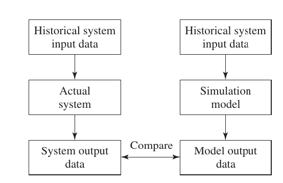
2. Confidence Intervals (The Statistical Standard)

This is the most reliable mathematical method. Instead of looking at a single number, you calculate a range (interval) for the difference ($D$) between the real-world mean ($m_S$) and the simulation mean ($m_M$).

$$\text{Confidence Interval} = \bar{D} \pm t_{\alpha/2, n-1} \frac{S_D}{\sqrt{n}}$$

The Rule of Zero: If the calculated range includes ‘0’ (Zero), it means there is no statistically significant difference between the real system and the simulation. Your model is statistically valid.

3. Time-Series Approaches

Simulation data is often “non-stationary,” meaning it changes over time.

Goal: This method checks if the patterns, trends, and cycles (e.g., peak hours in a bank) in the simulation match the timing and behavior of the real-world system over a specific period.

4. Turing Test (Qualitative Validation)

This is a “blind test” for experts. You present two unlabelled reports—one from the real system and one from the simulation—to managers or engineers.

Goal: If the experts cannot distinguish which report is which, the model is valid. If they can, their reasoning helps you find the logic errors in your code.

Continuous Systems

A Continuous System is one in which the state of the system changes continuously over time or with respect to another parameter, rather than in sudden, discrete jumps.

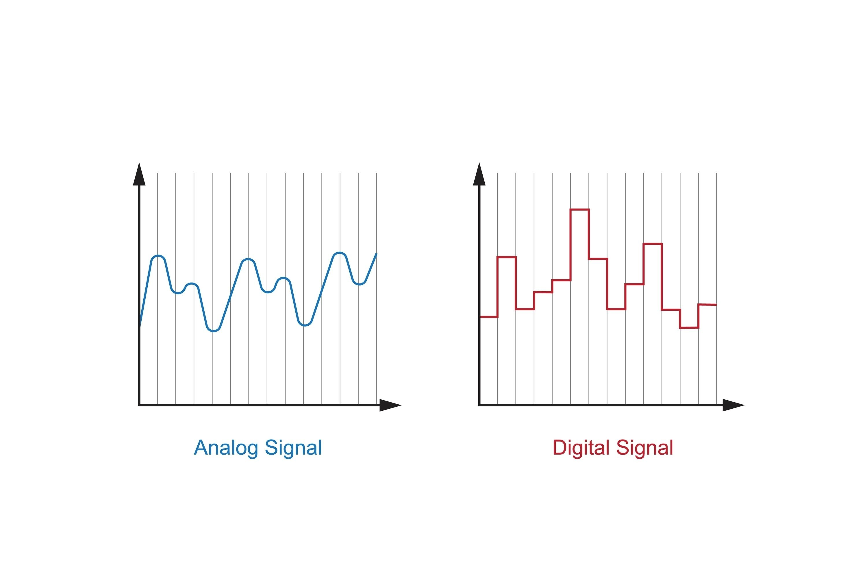
The image you uploaded perfectly illustrates the visual difference between Continuous and Discrete representations. In the context of system simulation, here is how these two graphs relate to the concepts we discussed:

1. Analog Signal (Continuous System)

Real-world Parallel: This is like a thermometer measuring temperature throughout the day; the mercury moves smoothly without “teleporting” from one degree to the next.

2. Digital Signal (Discrete System)

Real-world Parallel: This is like a digital clock that only changes when a full second passes. It “jumps” from 12:00:01 to 12:00:02 without showing the infinitesimal moments in between.

Pure Pursuit Problem

a pure pursuit scenario, a Pursuer (the chaser) like a fighter jet follows a Target (the leader) like bomber plane by always directing its velocity vector straight toward the target’s current position.

$(x_t - x_p)$: This represents the horizontal difference (left-to-right) between the two points.
$(y_t - y_p)$: This represents the vertical difference (up-to-down) between the two points.

the origin $(0, 0)$ and the target aircraft is at position $(3, 4)$.

$$D = \sqrt{(3 - 0)^2 + (4 - 0)^2}$$ $$D = \sqrt{3^2 + 4^2}$$ $$D = \sqrt{9 + 16}$$ $$D = \sqrt{25}$$ $$D = 5$$

View this post on Instagram

Real-time slab deflection analysis in action - Watch how the tool automatically processes BIM data and provides instant structural insights

Determining the Angle of Pursuit ($\sin \theta$ and $\cos \theta$)

To determine the angle at which the fighter aircraft must point itself toward the target, we use the following trigonometric formulas:

$$\sin \theta = \frac{y_b(t) - y_f(t)}{\text{Dist}(t)}; \quad \cos \theta = \frac{x_b(t) - x_f(t)}{\text{Dist}(t)}$$

These values tell the fighter jet exactly which direction to turn to remain locked onto the target’s current position.

Predicting the Next Position

To calculate the new coordinates of the fighter jet at the next time step ($t+1$), we use these equations:

$$x_f(t+1) = x_f(t) + S \cos \theta$$ $$y_f(t+1) = y_f(t) + S \sin \theta$$

Here, $S$ represents the speed of the fighter jet. This logic moves the fighter from its current position toward the target by a distance equal to its speed over that time interval.

Termination Conditions

The simulation continues step-by-step until one of the following two conditions is met:

Success: If the distance between the fighter and the bomber becomes 10 km or less, the pursuit ends, and the bomber is considered destroyed.
Failure: If the target’s path ends (e.g., after the 9th minute in your table) and the distance has not dropped below 10 km, the bomber is considered to have escaped, and the pursuit is called off.

3.3 Simulation of a Chemical Reaction

This simulation models a chemical reaction where two substances ($ch_1$ and $ch_2$) react to form a third substance ($ch_3$). This is a reversible reaction, meaning $ch_3$ can also break down back into its original components.

Core Reaction Formulas:

Forward Reaction: $ch_1 + ch_2 \rightarrow ch_3$
Backward Reaction: $ch_3 \rightarrow ch_1 + ch_2$

Mathematical Equations (Differential Equations):

The change in the quantity of these chemicals over time is expressed using the following differential equations:

$$\frac{dc_1}{dt} = k_2 c_3 - k_1 c_1 c_2$$
$$\frac{dc_3}{dt} = 2k_1 c_1 c_2 - 2k_2 c_3$$

Here, $k_1$ and $k_2$ are constants. These equations tell us exactly how the amounts of $c_1, c_2, \text{and } c_3$ increase or decrease at any given moment.

Simulation Methodology:

In the real world, these reactions occur so rapidly and complexly that calculating a direct result is difficult. Therefore, we use the “Small Time Increment” ($\Delta t$) method in simulations.

The Steps are:

Initial State: Define the quantity of chemicals at the start ($t=0$).
Time Step: Choose a very small interval of time ($\Delta t$).
Update Formula: Calculate the new amount of the substance after that small interval: $$c_1(t + \Delta t) = c_1(t) + \frac{dc_1(t)}{dt} \Delta t$$ (Meaning: New Amount = Current Amount + Rate of Change $\times$ Time)

1. Breakdown of the Formula

$c_1(t)$: Current amount of the substance.
$\frac{dc_1(t)}{dt}$: Rate of change. This indicates how much of the substance is being created or consumed per second.
$\Delta t$: A very small time step (e.g., 0.01 seconds).
$c_1(t + \Delta t)$: The updated amount of the substance at the next time step.

2. Practical Calculation Example

Imagine a container holds 100g of chemical $c_1$.

The rate of reaction ($\frac{dc_1}{dt}$) is -2 g/sec (it is negative because the substance is being consumed).
We want to find out how much remains after 0.5 seconds ($\Delta t$).

Calculation: $$c_1(\text{new}) = 100 + (-2 \times 0.5)$$ $$c_1(\text{new}) = 100 - 1$$ $$c_1(\text{new}) = 99 \text{ grams}$$

The reasons why determining the direct outcomes of chemical reactions

1. Speed of Reaction (High Speed)

Many chemical reactions occur in microseconds or even faster. In a laboratory, it is nearly impossible to track these lightning-fast changes with the naked eye or standard equipment. Simulation breaks time down into tiny increments ($dt$ or $\Delta t$), allowing us to see exactly what is happening at every moment.

2. Intermediate States

Between the start and the end of a reaction, many temporary states occur.

Example: Before $A + B \rightarrow C$ is completed, a very short-lived temporary substance called an “intermediate” might form. These are often impossible to capture physically, but simulations help us visualize these invisible steps.

3. Dynamic Concentration

During a reaction, the amounts of $ch_1$ and $ch_2$ decrease while $ch_3$ increases. The Rate of Change is not constant; it shifts every millisecond. Because the rate is constantly changing, using simple arithmetic to predict the amount of substance left after 10 minutes is extremely difficult. This requires Calculus and Differential Equations, which simulation software can solve with ease.

4. Environmental Factors

In the real world, temperature, pressure, and humidity are rarely perfectly stable. Controlling these in a lab is difficult and expensive. In a simulation, we can easily tweak these variables to see if a reaction will remain stable or become explosive.

5. Cost and Safety

Some chemical components are extremely expensive or dangerous (such as radioactive or toxic materials). Performing a simulation before a physical experiment ensures that the reaction is safe to conduct.

Exterior Ballistics.

Exterior Ballistics is the science that deals with the trajectory of a projectile (such as a bullet or cannonball) after it exits the firearm. Once a projectile is in flight, three primary forces act upon it:

Gravity: Pulls the object downward toward the earth.
Tangential Drag: The aerodynamic resistance of the air acting opposite to the direction of motion.
Air Resistance (Viscosity): A force proportional the velocity raised to a certain power ($kv^n$).

Equations of Motion (Differential Equations)

A projectile is launched at a specific angle ($\delta$) with an initial velocity. If the mass of the projectile is $m$, the forces along the tangent and normal directions are expressed by these two equations:

1. Tangential Equation: $$m \frac{dv}{dt} + mg \sin \theta + kv^n = 0$$ (This determines the rate at which the projectile’s velocity decreases over time.)

2. Normal Equation: $$m \frac{v^2}{\rho} + mg \cos \theta = 0$$ (This describes the curvature of the trajectory, where $\theta$ is the inclination of velocity and $\rho$ is the radius of curvature.)

1. Basic Kinematic Relations

Radius of Curvature ($\rho$): $\rho = \frac{ds}{d\theta}$. This describes how sharply the projectile’s path bends.
Velocity ($v$): $v = \frac{ds}{dt}$. This represents the rate of change of distance over time.

By combining these, the equation for the change in direction (the normal component of motion) becomes: $$mv\frac{d\theta}{dt} + mg \cos \theta = 0$$

2. Coordinate System

To track the projectile on a 2D map, we decompose the velocity into horizontal ($x$) and vertical ($y$) components:

$\frac{dx}{dt} = v \cos \theta$ (Horizontal displacement)
$\frac{dy}{dt} = v \sin \theta$ (Vertical displacement/Altitude)

3. The Simulation Algorithm (Step-by-Step)

Step 1: Initialization Set initial values: $v = v_0$ (muzzle velocity), $\theta = \phi$ (launch angle), $x = 0, y = 0$. Constants like mass ($m$), gravity ($g$), and the drag coefficient ($k$) are defined.

Step 2: Calculate Velocity Change ($\Delta v$) Compute how much the speed drops due to gravity and air resistance: $$\frac{\Delta v}{\Delta t} = -g \sin \theta - \frac{kv^n}{m}$$

Step 3: Calculate Directional Change ($\Delta \theta$) Determine how much the projectile “tilts” downward during that specific time interval: $$\frac{\Delta \theta}{\Delta t} = -g \frac{\cos \theta}{v}$$

Step 4: Calculate Positional Change ($\Delta x$ and $\Delta y$) Calculate the small distance moved in the $x$ and $y$ directions: $$\Delta x = (v \cos \theta) \Delta t \quad \text{and} \quad \Delta y = (v \sin \theta) \Delta t$$

Step 5: Update State Add the changes to the previous values to get the new state:

$v_{new} = v_{old} + \Delta v$
$x_{new} = x_{old} + \Delta x$ (and so on for $\theta$ and $y$)

Step 6: Iteration (The Loop) Repeat Steps 2 through 5 continuously until the projectile hits the ground (when $y \leq 0$).

The Role of Simulation

While simple projectile motion can be solved by hand, adding complex factors like variable air resistance ($kv^n$) makes it nearly impossible to solve using standard calculus. Simulation and Numerical Methods are used to calculate the projectile’s position ($x, y$) and velocity at extremely small time intervals. In simple terms, this simulation allows us to predict exactly where a cannonball will land by accounting for both gravity and air resistance.

3.8 Analog Simulation

Analog simulation is a process where a mathematical model of a physical system is represented and solved using analog electronic circuits (typically using voltage as the representing medium).

Key Features

Variable Representation: In this method, real-world physical variables (such as velocity, pressure, or temperature) are represented by continuous electrical voltages.
Core Hardware: The primary component used to perform mathematical operations like addition, subtraction, multiplication, or integration is the Operational Amplifier (Op-Amp).
Block-Based Design: Each mathematical function is treated as a separate “block.” These blocks are interconnected with wires to build the complete model of the physical system.
Continuous Results: Unlike digital computers that provide discrete data points, analog simulations provide a continuous stream of results, allowing for real-time observation of changes.

Disadvantages of Analog Simulation

Limited Accuracy: The precision of the results is dependent on the quality and tolerance of the electrical components (resistors, capacitors), making it less accurate than digital computers.
Magnitude Scaling: Since the operating voltage is limited (e.g., -10V to +10V), it is difficult to represent very large or very small numerical values without complex scaling.
Hardware Reconfiguration: Every time a new problem needs to be solved, the physical circuit must be rewired or rebuilt, which is time-consuming compared to simply changing a few lines of code.

For your exam preparation, here is the English translation and a structured breakdown of the concepts regarding Random Numbers in simulation. This is written in a professional, academic style suitable for your CSE courses.

4.1 Random Numbers

Random numbers are an essential component in computer simulation, particularly when using the Monte Carlo method. Many real-world systems produce results that depend on chance or uncertainty; these are known as Stochastic Systems. To model such systems accurately, we must utilize random numbers.

Definition

A Random Number is a value chosen from a specific interval where the distribution is uniform, and every possible number within that range has an equal probability of being selected.

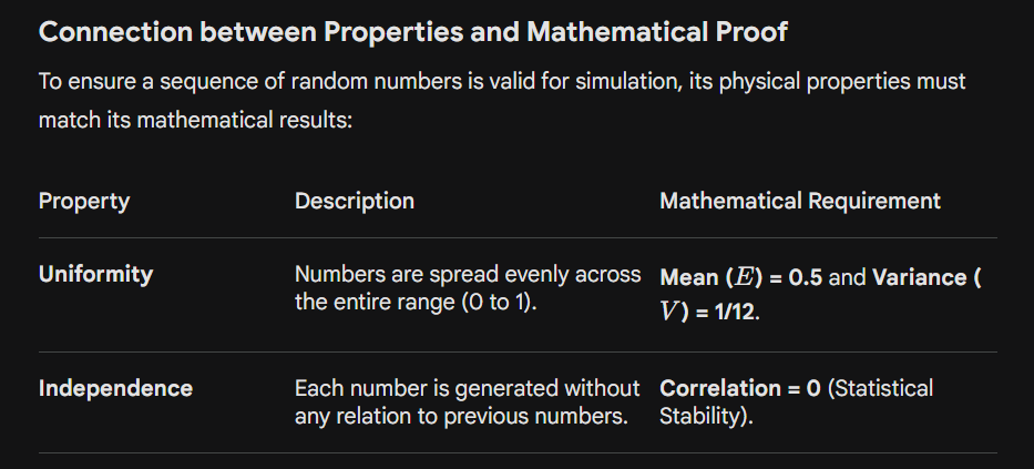
Properties of Random Numbers

A high-quality sequence of random numbers must satisfy two primary statistical properties:

1. Uniformity

The numbers must be distributed evenly across the entire defined range (usually between 0 and 1). This means if you divide the range into sub-intervals, each interval should contain approximately the same number of data points.

2. Independence

The occurrence of one number must not have any correlation or relationship with the numbers that came before it or the numbers that follow it. In other words, knowing the current random number should give you zero information about what the next number will be.

পরীক্ষায় র‍্যান্ডম নাম্বারের নির্ভরযোগ্যতা বা পরিসংখ্যানগত বৈশিষ্ট্য (Statistical Properties) যাচাই করার জন্য এই দুটি গাণিতিক মান খুবই গুরুত্বপূর্ণ। নিচে এটি ইংরেজিতে সহজভাবে উপস্থাপন করা হলো:

2. Principal Mathematical Values for Randomness

To verify if a set of generated random numbers (distributed between $0$ and $1$) is truly uniform, two primary statistical measures are used:

A. Expected Value or Mean, $E(R)$

The Expected Value represents the average of the random numbers in the sequence. For a perfectly uniform distribution between $0$ and $1$, the mean should always be 0.5.

The Formula: $$E(R) = \int_{0}^{1} x , dx = \left[ \frac{x^2}{2} \right]_0^1 = \frac{1}{2} = 0.5$$

B. Variance, $V(R)$

The Variance measures the spread of the numbers around the mean. It tells us how far the numbers are scattered from $0.5$. For a uniform sequence, the variance is always 1/12 (approximately $0.0833$).

The Formula: $$V(R) = \int_{0}^{1} x^2 , dx - [E(R)]^2$$ $$V(R) = \left[ \frac{x^3}{3} \right]_0^1 - (0.5)^2 = \frac{1}{3} - \frac{1}{4} = \frac{1}{12}$$

Checking

If your simulation’s random numbers have an average far from $0.5$, the sequence is biased.
If the variance is significantly different from $1/12$, the sequence is not uniformly distributed (i.e., numbers might be clustering in one area).

Pseudo-random Numbers:

are sequences of numbers that appear to be random but are actually generated using a specific mathematical formula or algorithm.Because they follow a deterministic formula, if you start with the same “Seed” (the initial starting value), you will always get the exact same sequence of numbers. This is why they are called “Pseudo” (fake) random.

The Linear Congruential Method (LCM)

This is the most common algorithm for generating pseudo-random numbers. The general formula is:

$$X_{i+1} = (aX_i + c) \mod m$$

Practical Example

Let’s calculate the first 3 numbers using these parameters:

Seed ($X_0$): $27$ (Starting value)
Multiplier ($a$): $17$
Increment ($c$): $43$
Modulus ($m$): $100$ (Results will stay between $0$ and $99$)

Step 1: Finding $X_1$ $$X_1 = (17 \times 27 + 43) \mod 100$$ $$X_1 = (459 + 43) \mod 100 = 502 \mod 100 = 2$$ First Random Number: 2

Step 2: Finding $X_2$ (using $X_1 = 2$) $$X_2 = (17 \times 2 + 43) \mod 100$$ $$X_2 = (34 + 43) \mod 100 = 77 \mod 100 = 77$$ Second Random Number: 77

Step 3: Finding $X_3$ (using $X_2 = 77$) $$X_3 = (17 \times 77 + 43) \mod 100$$ $$X_3 = (1309 + 43) \mod 100 = 1352 \mod 100 = 52$$ Third Random Number: 52

Resulting Sequence: $2, 77, 52 \dots$

Why are Pseudo-random Numbers Important?

Repeatability: If you use the same Seed ($X_0 = 27$) again, you get the exact same sequence. This is vital for debugging simulations.
Efficiency/Speed: These algorithms are computationally very fast and require very little memory.
Uniformity: A well-chosen $a, c,$ and $m$ ensure that the numbers are spread evenly across the interval.

Departures from Ideal Randomness

Non-Uniformity: The numbers are not spread evenly; they might cluster in certain areas.
Discontinuity: There are large gaps between numbers instead of a smooth range.
Mean Error: The average (Mean) of the numbers is significantly higher or lower than 0.5.
Variance Error: The spread (Variance) is not 1/12, meaning the numbers are either too close together or too scattered.
Cyclic Patterns: The sequence repeats the same numbers after a short period (e.g., $1, 5, 9, 1, 5, 9…$).
Correlation: A number might depend on the one before it, meaning the sequence is not truly independent.

A Random Number Table

is a statistically generated, printed list of digits (0–9) arranged in rows and columns, designed to ensure each digit is equally likely to be chosen and independent of others.

Here is a simplified and short English version of the methods and their limitations, perfect for quick exam revision:

Methods of Generating Random Numbers

There are three ways to get random numbers for simulations:

A. Random Number Tables:
- What it is: Pre-made lists stored in memory.
- Drawback: Very slow and uses too much storage.
B. Electronic Devices:
- What it is: Special hardware that generates “True” random numbers.
- Drawback: Very expensive to build and maintain.
C. Pseudo-Random Numbers:
- What it is: Generated using math formulas (Algorithms).
- Process: Starts with a Seed; each number calculates the next.
- Best Part: It is the most popular method because it is fast and repeatable.

Stochastic System:

A system that involves a random variable, making its behavior unpredictable even if the initial conditions are known.

Mid-Square Random Number Generator

The Mid-Square method is one of the oldest ways to generate pseudo-random numbers. It was used in the 1950s for early nuclear simulation designs.

How it works (Steps):

Choose a Seed: Pick an $n$-digit number (e.g., a 4-digit number).
Square it: Calculate the square of the number.
Extract Middle: Take the middle $n$ digits of the result. This is your new random number.
Repeat: Use this new number as the seed for the next step.

Example:

Seed ($n=4$): $5673$
Square: $32,182,929$ (8 digits)
Middle 4 digits: $1829$ (Next Random Number)

Limitations (The “Degeneracy” Problem)

As shown in your slides (image_af721c.jpg), this method is rarely used today because it is unstable:

Degeneracy to Zero: The sequence often results in $0000$. Once it hits zero, every following number will also be zero.
- Example: Seed $2061$ eventually leads to all zeros.
Stagnation (Constant): The sequence can get stuck on a single number.
- Example: $2500^2 = 06,250,000$. The middle 4 digits are $2500$ again.
Short Loops: The generator may get stuck in a tiny loop (e.g., $2100 \rightarrow 4100 \rightarrow 8100 \rightarrow 6100 \rightarrow 2100 \dots$).
Limited Sequence: It cannot provide the millions of unique numbers required for modern, large-scale simulations.

Congruence (Residue) Method

This is the most popular method for generating pseudo-random numbers in modern computers.

The Formula

The next random number is calculated using this modular arithmetic equation: $$r_{i+1} = (ar_i + b) \mod m$$

$r_0$: The Seed (starting value).
$a$: Multiplier.
$b$: Increment.
$m$: Modulus (defines the range and the period).
$\text{mod } m$: This takes the remainder after division.

Types of Congruence Methods

Type	Condition	Formula
Mixed Method	$a > 1, b > 0$	$r_{i+1} = (ar_i + b) \mod m$
Additive Method	$a = 1$	$r_{i+1} = (r_i + b) \mod m$
Multiplicative Method	$b = 0$	$r_{i+1} = (ar_i) \mod m$

Note: The Multiplicative Method is generally considered more efficient than the Additive method and as effective as the Mixed method.

Normalizing the Output ($0$ to $1$)

Since the formula produces integers (like $14, 12, 5$), we must convert them into decimals between 0 and 1 for simulation use: $$R_i = \frac{r_i}{m}$$

Example Calculation

Given: $a=13, b=1, m=19,$ and $r_0=1$.

$r_1$: $(13 \times 1 + 1) \mod 19 = 14 \mod 19 = \mathbf{14}$ $\rightarrow R_1 = \mathbf{0.7368}$
$r_2$: $(13 \times 14 + 1) \mod 19 = 183 \mod 19 = \mathbf{12}$ $\rightarrow R_2 = \mathbf{0.6316}$

Limitation: The Period

The main limitation is that the sequence will eventually repeat. The maximum number of unique values it can produce is equal to $m$.

In your example ($m=19$), the sequence repeats after 18 or 19 numbers.
In modern computers, $m$ is set to very large values like $2^{31}-1$, ensuring the sequence doesn’t repeat for billions of steps.

4.7 Arithmetic Congruential Generator

This method generates pseudo-random numbers by adding previous values in the sequence, similar to how the Fibonacci sequence works.

The Formula

To find the next number ($r_{i+1}$), you add the two previous numbers and take the modulus: $$r_{i+1} = (r_{i-1} + r_i) \mod m$$

How it Works (Steps):

Two Seeds: Unlike other methods, this requires two initial starting numbers ($r_1$ and $r_2$).
Addition: Add the current number to the previous one.
Modulus: Take the remainder after dividing by $m$.

Practical Example:

Given: $r_1 = 9, r_2 = 13,$ and $m = 17$.

Find $r_3$: $(9 + 13) \mod 17 = 22 \mod 17 = \mathbf{5}$
Find $r_4$: $(13 + 5) \mod 17 = 18 \mod 17 = \mathbf{1}$
Sequence: $9, 13, 5, 1 \dots$

Key Advantages:

Speed: It is computationally very fast because addition is faster than multiplication (unlike the LCM method).
Long Period: If the seeds and modulus are chosen carefully, it can produce a very long sequence of numbers before repeating.

This is an excellent summary of why we use Combined Congruential Generators (CCG). When a single generator isn’t “random” enough or repeats too quickly, combining them is the perfect solution. Here is the simplified English version for your notes:

Combined Congruential Generators (CCG)

A single generator often has a short “period” (it starts repeating too soon). To solve this, we combine multiple independent generators to create a sequence with a much longer period and better statistical properties.

Key Advantages

Massive Period: It can generate billions of unique numbers before repeating.
Higher Quality: The combined sequence passes stricter statistical tests for randomness than any single generator could.

Mathematical Requirements

Modulus ($m$): Should be a large Prime Number to maximize the range.
Multiplier ($a$): Should be a Primitive Root of $m$ to ensure the generator reaches its full potential (maximum period).
Normalization: To get values between 0 and 1, the final result is divided by the modulus ($R_i = r_i / m$).

Real-World Example: LeEcuyer’s Generator

Researcher Pierre L’Ecuyer showed that by combining just two simple generators, we can achieve a period of approximately 2 billion ($2 \times 10^9$) numbers.

Regarding the Period formula: Yes, let’s look at it briefly. The formula you mentioned: $$P = \frac{(m_1-1)(m_2-1)\dots}{2^{k-1}}$$

This summary perfectly captures the industry standards for evaluating a generator. For your exams, here is the short and simple English version:

Qualities of an Efficient Random Number Generator

A high-quality generator must meet the following criteria to be useful in professional simulations:

Long Cycle (Period): It should generate a massive number of unique values before the sequence repeats itself.
Replicability: Using the same Seed must produce the exact same sequence. This is essential for debugging and comparing different simulation models.
Statistical Accuracy: The numbers must strictly follow the properties of Uniformity (even spread) and Independence (no patterns).
Efficiency: It must be fast and consume minimal computer memory (RAM).
Portability: The algorithm should work consistently across different programming languages and hardware systems.

Testing Numbers for Randomness

Before using a sequence in a simulation, it must pass two critical tests:

1. The Uniformity Test

Every number in the defined range must have an equal probability of appearing. For example, if you generate 1,000 numbers between 0 and 9, each digit (0, 1, 2…) should appear roughly 100 times.

2. The Independence Test (No Auto-correlation)

There should be no relationship between consecutive numbers. If you can predict the next number based on the current one, the sequence is not random.

Example of Fail: $1, 3, 5, 7, 9 \dots$ (This fails because there is a clear mathematical pattern).

For your exams, you can summarize the Uniformity Test in these simple points:

4.11 Uniformity Test

The Uniformity Test is the most basic way to check if a random number generator is working correctly. It verifies if the generated numbers are spread evenly across the expected range (usually 0 to 1).

The Goal

To see if the observed frequency (the numbers we actually got) matches the theoretical frequency (what we expected to get).

Main Testing Methods

There are two primary “Frequency Tests” used for this purpose:

Kolmogorov-Smirnov Test (K-S Test): * This compares the cumulative distribution of the sample with the theoretical uniform distribution.
- It is generally preferred for small sample sizes.
Chi-Square Test ($\chi^2$ Test): * This divides the range into several “bins” or intervals and counts how many numbers fall into each bin.
- It is the most common method and is better suited for large sample sizes.

The Chi-square Test ($\chi^2$) is

the most widely used statistical method to check the Uniformity of random numbers, especially when dealing with large datasets ($N > 50$).The test divides the range (0 to 1) into equal intervals (bins). It compares the Observed Frequency ($O_i$ — how many numbers actually fell into a bin) with the Expected Frequency ($E_i$ — how many numbers should have fallen into that bin if they were perfectly uniform).

2. The Formula

$$\chi^2_0 = \sum_{i=1}^{n} \frac{(O_i - E_i)^2}{E_i}$$

$n$: Number of intervals.
$O_i$: Observed count in interval $i$.
$E_i$: Expected count ($E_i = N/n$, where $N$ is total numbers).

3. Steps to Perform the Test

Example: $N = 100$ numbers, $n = 10$ intervals. Thus, $E_i = 100/10 = 10$.

Step 1 (Count): Count how many numbers fall into each interval (e.g., $0.0-0.1$ has 8, $0.1-0.2$ has 12).

Actual numbers found: 8 (e.g., $0.02, 0.05, 0.09 \dots$)

Step 2 (Calculate): Plug the values into the formula: $\frac{(8-10)^2}{10} + \frac{(12-10)^2}{10} + \dots$
Step 3 (Degrees of Freedom): Calculate $df = n - 1$. For 10 intervals, $df = 9$.
Step 4 (Decision): Compare your calculated $\chi^2_0$ with the Critical Value from a standard Chi-square Table.

Decision Rule: > * If $\chi^2_0 < \text{Critical Value}$: The numbers are Uniform (Accept).
If $\chi^2_0 > \text{Critical Value}$: The numbers are Not Uniform (Reject).

4. Comparison: K-S Test vs. Chi-square Test

Feature	K-S Test	Chi-square Test
Sample Size	Best for small samples ($N < 20$).	Best for large samples ($N > 50$).
Method	Compares every single number.	Groups numbers into intervals.
Sensitivity	Very sensitive and precise.	Slightly less sensitive but easier for big data.

These two tests are critical for proving Independence (Autocorrelation Test) and Internal Randomness (Poker Test). Here is the short and simple English breakdown for your exam preparation:

4.13 Testing for Autocorrelation

Uniformity is not enough. A sequence like $0.1, 0.2, 0.3 \dots$ is perfectly uniform but not random because each number depends on the one before it. This is called Serial Correlation.

How it is tested:

The Matrix Method: We use a $10 \times 10$ matrix (checkerboard).
Pairs: We take pairs of numbers (like $X_i$ and $X_{i+1}$) and plot them as coordinates on the grid.
The Goal: If the dots are scattered randomly across the grid, the sequence is independent. If the dots form lines or patterns, the sequence fails.
Simplified Classes: Sometimes, instead of 10 divisions, we use 3 broad classes (e.g., Low $\le 0.33$, Mid $\le 0.67$, High $\le 1.0$) to make the calculation faster.

4.14 The Poker Test

Named after the card game, this test looks inside the digits of a single random number to see if the digits themselves are distributed randomly.

How it works:

Each number is treated as a 5-digit “Hand.” For example, if the number is $0.71549$, the hand is $[7, 1, 5, 4, 9]$. We then categorize these digits just like Poker hands:

Category	Example	Probability (Approx.)
All Different	$71549$	~30.24%
One Pair	$55137$	~50.40%
Two Pairs	$33669$	~10.80%
Three of a Kind	$55513$	~0.72%
Full House	$44477$	~0.09%
Four of a Kind	$77774$	~0.045%
Five of a Kind	$88888$	~0.01%