Simulation And Modeling
Another alll example provide this link
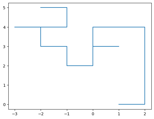
Rnadom Walk problem
import math
import random
import matplotlib.pyplot as plt
for asa in range(1):
    step = 0
    x = 0
    y = 0
    dotx = []
    doty = []
    direction = []

    F_L_R = [0.5, 0.2, 0.2, 0.1]
    F_L_R = [int(10 * i) for i in F_L_R] ## F_L_R: [5, 2, 2, 1]।

    while step <= 20:

        rn = random.randint(0, 9)

        if rn in range(F_L_R[0]): ## Forward	range(0, 5)	actual value is= 0, 1, 2, 3, 4
            direction.append('F')
            y += 1
            dotx.append(x)
            doty.append(y)
        elif rn in range(F_L_R[0], F_L_R[0] + F_L_R[1]):
            direction.append('L')
            x -= 1
            dotx.append(x)
            doty.append(y)
        elif rn in range(F_L_R[1],F_L_R[0]+ F_L_R[1]+F_L_R[2]): ## Right	range(7, 9) actual value is= 7,8
            direction.append('R')
            x += 1
            dotx.append(x)
            doty.append(y)
        else:
            y -= 1
            direction.append('B')
            dotx.append(x)
            doty.append(y)
        step += 1
    plt.plot(dotx, doty)
plt.show()
Relability problem
- This section sets up the “Wheel of Fortune” ranges for the simulation.
import math
import random
import matplotlib.pyplot as plt

# --- Data Setup ---
life = [1000, 1100, 1200, 1300, 1400, 1500, 1600, 1700, 1800, 1900]
probability = [0.10, .14, .24, .14, .12, .10, .06, .05, .03, 0.02]
probability = [int(i * 100) for i in probability]

# Create Cumulative Probability for Bearing Life
c_probability = [probability[0]]
for i in range(1, len(probability)):
    c_probability.append(c_probability[i - 1] + probability[i])

# Create Cumulative Probability for Mechanic Delay
delay = [4, 6, 8]
delay_probability = [0.3, 0.6, 0.1]
delay_probability = [int(i * 10) for i in delay_probability]

# delay = [4, 6, 8] (minute)
# delay_probability = [3, 6, 1] (after integer number)

c_delay_pro = [delay_probability[0]]
for i in range(1, len(delay_probability)):
    c_delay_pro.append(c_delay_pro[i - 1] + delay_probability[i])
- Random Selection Functions
def clock():
    """Returns a random bearing life based on probability distribution."""
    x = random.randint(1, 100)
    for index, cum_prob in enumerate(c_probability):
        if x <= cum_prob:
            return life[index]
    return life[-1]
   # return life[-1]: if loop not obey this condition then retuen last largest value

def late():
    """Returns a random mechanic delay time."""
    x = random.randint(1, 10)
    for index, cum_prob in enumerate(c_delay_pro):
        if x <= cum_prob:
            return delay[index]
    return delay[-1]
- Individual Replacement
# --- Simulate 20,000 hours for 3 separate bearings ---
bearing1_life, bearing2_life, bearing3_life = [], [], []

for history_list in [bearing1_life, bearing2_life, bearing3_life]:
    lf = 0
    while lf < 20000:
        val = clock()
        lf += val
        history_list.append(val)

# Calculate coincidental failures (if they break at the same interval)
bearing_life_count = [len(bearing1_life), len(bearing2_life), len(bearing3_life)]
maxlen = max(bearing_life_count)
two_down, three_down = 0, 0  # initial declare variables

for i in range(maxlen):
    try:
        b1, b2, b3 = bearing1_life[i], bearing2_life[i], bearing3_life[i]
        if b1 == b2 == b3:
            three_down += 1
        elif b1 == b2 or b2 == b3 or b3 == b1:
            two_down += 1
    except IndexError: # try-except: If one list contains 10 data and the other contains 12 data, this is used to avoid index errors.
        pass

# --- Cost Calculation for Policy 1 ---
num_of_bearing = sum(bearing_life_count)
total_bearing_cost = num_of_bearing * 20

# Delay costs (fewer calls if bearings fail together)
num_of_mechanic_call = num_of_bearing - two_down - (three_down * 2) # Only 1 call is needed instead of 3 calls (2 calls saved). So three_down * 2 is subtracted.
total_delay_cost = sum([late() for _ in range(num_of_mechanic_call)]) * 5

# Repair time: 20m per bearing, 10m saved for double, 20m saved for triple
time_needed = (num_of_bearing * 20) - (two_down * 10) - (three_down * 20)
total_repair_cost = (time_needed / 60) * 25

total_cost_1 = total_bearing_cost + total_delay_cost + total_repair_cost
- Group Replacement
bearing_life_group = []
mechanic_delay_group = []
lf = 0

while lf < 20000:
    # All 3 are checked, but the machine stops at the first failure
    life_of_bearings = [clock(), clock(), clock()]
    shortest_life = min(life_of_bearings)

    bearing_life_group.append(shortest_life)
    mechanic_delay_group.append(late())
    lf += shortest_life

# --- Cost Calculation for Policy 2 ---
# We replace 3 bearings every time the machine stops
total_bearing_cost_2 = (len(bearing_life_group) * 3) * 20  # Only 1 call is needed instead of 1 calls
total_delay_cost_2 = sum(mechanic_delay_group) * 5

# Group repair is faster: roughly 40 mins total for all three
total_repair_cost_2 = ((len(bearing_life_group) * 40) / 60) * 25
# Once the mechanic comes and replaces 3 bearings at once it takes less time (only 40 minutes
# instead of 20 minutes to 60 minutes each).
total_cost_2 = total_bearing_cost_2 + total_delay_cost_2 + total_repair_cost_2

# --- Final Results ---
print(f"Policy 1 (Individual) Cost: ${total_cost_1:.2f}")
print(f"Policy 2 (Group) Cost:      ${total_cost_2:.2f}")
print(f"Total Savings:             ${total_cost_1 - total_cost_2:.2f}")
Simulation of Bombing problem
import random
import numpy as np
import matplotlib.pyplot as plt
length = 1000
height = 600

deviation_x = length / 2
deviation_y = height / 2
def getRNN():
    rnn = np.random.randn()
    return rnn
HIT = 0
N = 0

for i in range(100):
    x = getRNN() * deviation_x
    y = getRNN() * deviation_y
    N += 1
    if (x <= length/2 and x >= -length/2) and (y <= height/2 and y >= -height/2):
        HIT += 1
        plt.scatter(x,y,color = "green")
    else:
        plt.scatter(x,y,color = "blue")


area_x = [-500, 500, 500, -500, -500]
area_y = [-300, -300, 300, 300, -300]
(-500, -300): Lower left corner.
(500, -300): Lower right corner.
(500, 300): Upper right corner.
(-500, 300): Upper left corner.
(-500, -300): Return to the beginning (to close the line).
plt.plot(area_x, area_y, color="red")
plt.show()

print(HIT, N)
print("Accuracy : ", (HIT / N) * 100, "%")
-- Exam Question 2023 (session 2020-2021)--
- A six-sided die rolled and produces random numbers 1 to 6. Simulate the Gambling Game with six-sided die rolled in odd trail is treated as H and even trail as T. When the differences between H and T will 20 game over. It costs 1 dollar in each trail. Use Monte Carlo Method and analyze profit-loss. (08)
import random

def simulate_gambling_game():
    """
    Simulates a Gambling Game using Monte Carlo Method.
    The game continues until the difference between 'H' and 'T' reaches 20 or more.
    Each trial costs $1.
    """

    h_count = 0      # Count of Heads (H) - Odd numbers
    t_count = 0      # Count of Tails (T) - Even numbers
    trails = 0       # Total number of trials (dice rolls)
    cost_per_trial = 1  # Cost per trial in dollars

    # Continue the game until the absolute difference between H and T is 20 or more
    while abs(h_count - t_count) < 20:
        trails += 1
        # Simulate rolling a die (1 to 6)
        die_roll = random.randint(1, 6)

        # If the number is odd → it's H (Heads)
        if die_roll % 2 != 0:
            h_count += 1
        # If the number is even → it's T (Tails)
        else:
            t_count += 1

    # Calculate total cost
    total_cost = trails * cost_per_trial

    # Display simulation results
    print(f"--- GAMBLING GAME SIMULATION RESULT ---")
    print(f"Total Trails (Dice Rolls): {trails}")
    print(f"Number of H (Odd): {h_count}")
    print(f"Number of T (Even): {t_count}")
    print(f"Final Difference |H - T|: {abs(h_count - t_count)}")
    print(f"Total Cost: ${total_cost}")

    # Profit-Loss Analysis
    # Assuming the player wins $50 prize if the game ends
    prize = 50
    profit_loss = prize - total_cost

    if profit_loss > 0:
        print(f"Profit: +${profit_loss}")
    elif profit_loss < 0:
        print(f"Loss: -${abs(profit_loss)}")
    else:
        print(f"Break Even: $0")


# Run the simulation
simulate_gambling_game()
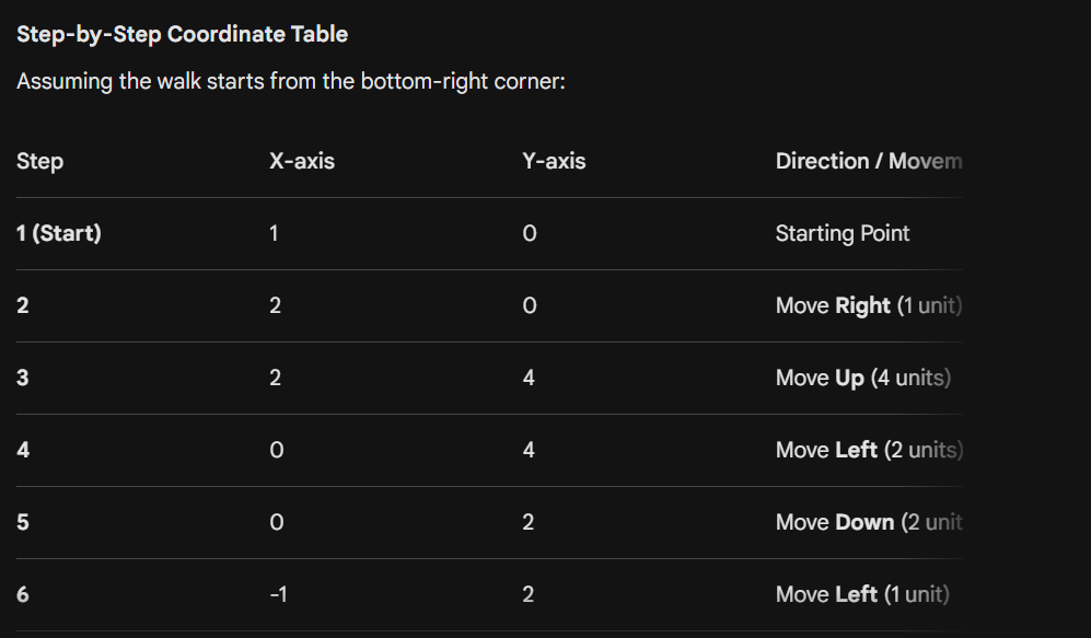
- A flying object moves randomly. It moves L, R, F and B in 25%, 35%, 30% and 10% probability. It also has 80% upward and 20% downward tendency. Identify the location of flying object after 50 epochs by Monte Carlo Method. (08)
import random

def simulate_flying_object(epochs=50):
    # Initialize starting coordinates (x, y, z)
    # x: Left/Right, y: Forward/Backward, z: Up/Down
    x, y, z = 0, 0, 0

    for i in range(1, epochs + 1):
        # 1. Horizontal Movement (L, R, F, B)
        # Probabilities: L=25%, R=35%, F=30%, B=10%
        # We use a random number between 1 and 100 to pick the direction
        horizontal_rand = random.randint(1, 100)

        if horizontal_rand <= 25:
            x -= 1  # Move Left
        elif horizontal_rand <= 60: # 25 + 35
            x += 1  # Move Right
        elif horizontal_rand <= 90: # 60 + 30
            y += 1  # Move Forward
        else:
            y -= 1  # Move Backward

        # 2. Vertical Movement (Upward/Downward)
        # Probabilities: Up=80%, Down=20%
        vertical_rand = random.randint(1, 100)

        if vertical_rand <= 80:
            z += 1  # Move Upward
        else:
            z -= 1  # Move Downward

    return x, y, z

# Execute the simulation for 50 epochs
final_x, final_y, final_z = simulate_flying_object(50)

# Display the results
print(f"--- Simulation Results after 50 Epochs ---")
print(f"Final Coordinates: (x: {final_x}, y: {final_y}, z: {final_z})")
print(f"Total Horizontal Displacement: x={final_x}, y={final_y}")
print(f"Total Vertical Altitude: z={final_z}")
--- Simulation Results after 50 Epochs ---
Final Coordinates: (x: 7, y: 13, z: 28)
Total Horizontal Displacement: x=7, y=13
Total Vertical Altitude: z=28
Let's say the initial position is $(0, 0, 0)$.
1. Epoch 1: Random number (42, 15) is generated.
o $x = +1$ for 42 (R).
o $z = +1$ for 15 (Up).
o New position: $(1, 0, 1)$.
Write a program that performs a simple M/M/1 queue simulation. This program requires parameters for the Mean Inter Arrival time of customers, Mean Service time as well as the maximum number of customers. The simulation is started with a single-server queue with a FIFO queuing discipline. For M/M/1 queue, the customer inter-arrival time and the service time are both exponentially distributed. This simulation shows the Average delay in queue, Average number in queue, Server utilization, and Time simulation ended. (07)
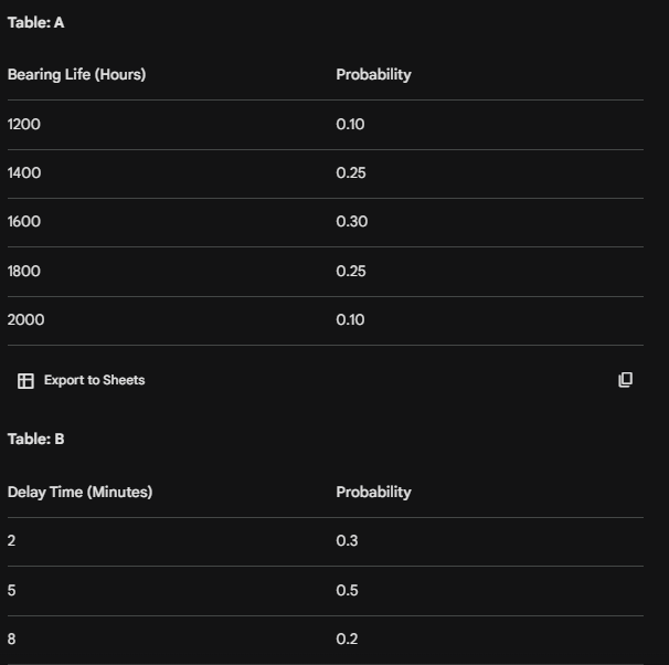
-- Exam Question 2023 Final exam (session 2020-2021)--A machine center has three identical bearings, which fail according to the following probability distribution in table A. The present maintenance policy is to change a bearing as and when it fails. When bearing fails machine center stops, a technician is called to replace the failed bearing with a new one. The time between the failure of the bearing and reporting of the technician (delay time) is random and is distributed as table B.
-- Exam Question 2021 (session 2018-2019)--
- Calculate the area of an irregular figure by Monte Carlo Method.
- Simulate the Gambling Game by Monte Carlo Method and analyze profit-loss.
- Find the value of a numerical integration by Monte Carlo Method of any differential equation.
- Determination of the value of π by Monte Carlo Method.
- Solve Random walk by Monte Carlo Method.
- Simulate Reliability Problem.
- Implement Kolmogorov test with midsquare random numbers.
- Implement Chi-Square test with multiplicative congruential random numbers.
- Implement chi-square test for autocorrelation with additive congruential random numbers.
- Implement poker test with multiplicative congruential random numbers.