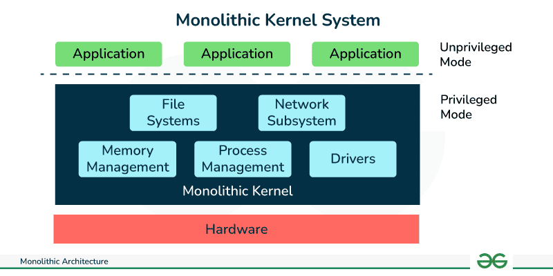
Fig. 2.6 & 2.7: A dongle is a small, portable hardware device that plugs into a port (usually USB or HDMI) on a computer or other electronic device to provide additional features or functionality.
Fig. 2.6 & 2.7: A dongle is a small, portable hardware device that plugs into a port (usually USB or HDMI) on a computer or other electronic device to provide additional features or functionality.
Fig. 2.6 & 2.7: A dongle is a small, portable hardware device that plugs into a port (usually USB or HDMI) on a computer or other electronic device to provide additional features or functionality.
Fig. 2.6 & 2.7: A dongle is a small, portable hardware device that plugs into a port (usually USB or HDMI) on a computer or other electronic device to provide additional features or functionality.
Fig. 2.6 & 2.7: A dongle is a small, portable hardware device that plugs into a port (usually USB or HDMI) on a computer or other electronic device to provide additional features or functionality.
Fig. 2.6 & 2.7: A dongle is a small, portable hardware device that plugs into a port (usually USB or HDMI) on a computer or other electronic device to provide additional features or functionality.
1. Define Program and Process
A program is sitting in computer storage (Hard Drive), it is simply a passive entity that is progaram (e.g., Chrome.exe).The moment you open it and it begins to execute, it becomes an active entity known as a ‘Process.’.It has a Program Counter to track which instruction to execute next.
Early Computers: Older computer systems allowed only one program to run at a time. That single program had complete control over all system resources.
Modern Computers: Contemporary systems can run multiple programs simultaneously (e.g., listening to music while typing a document). This capability is known as Concurrency.
When you use a computer or phone today, you run many apps or programs simultaneously (such as a browser, email, and typing software). Even if a small device is running only a single program, the operating system still has to perform its own internal tasks, such as memory management, in the background.All these types of tasks—Known as Process.
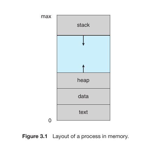
Layout of a Process in Memory
How a Process is positioned or mapped within the system memory. This is a fundamental concept in Operating Systems. When a program is loaded into memory (RAM) as a process, it is primarily divided into four sections:
Section
Purpose
Text
This contains the executable instructions or the actual code of the program. It is usually read-only to prevent accidental modification of the code.
Data
This section stores global variables and static variables that are defined outside of functions.
Heap
This is dynamic memory. It is used for memory allocation during run-time (for example, using malloc in C or new in Java/C++).
Stack
This holds temporary data, such as function parameters, local variables, and return addresses. Used for function calls. Whenever a function is invoked, is pushed onto the stack. When the function finishes, it is popped (removed).
Fixed Sections: The Text and Data sections are static Dynamic Sections: The Stack and Heap are flexible and change size
Fig.1
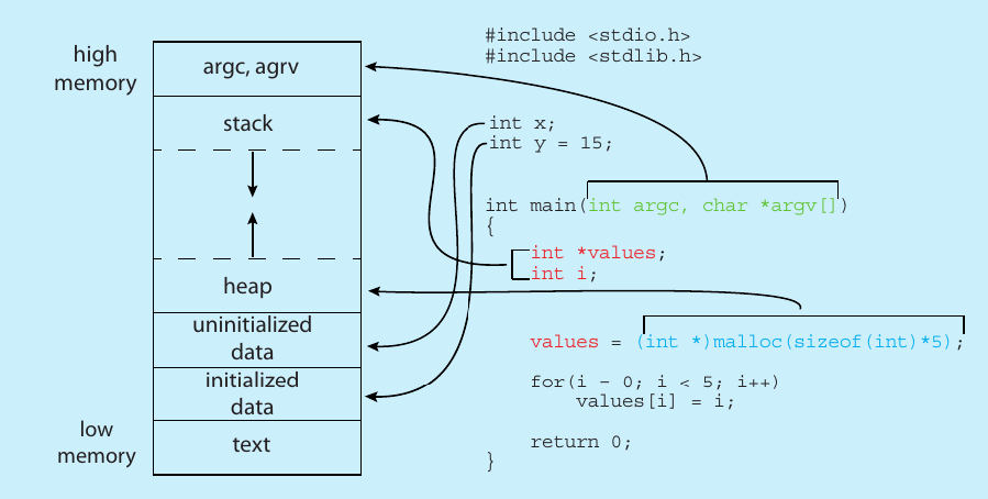
C program storing in Memory when acts as a process
Text Section
Stores the compiled machine instructions. For example, the logic written inside your main() function is stored here as binary code.
Initialized Data
This section stores global and static variables that have been assigned a value by the programmer in the source code.
Example:int y = 15; defined outside a function.
Uninitialized Data (BSS): Stores global or static variables that are declared but not assigned a value (e.g., int x;). BSS stands for Block Started by Symbol.
Heap: This is for dynamic memory. When you use malloc() to request memory while the program is running, that space is carved out of the Heap.
Stack: Stores local variables defined inside functions (e.g., int i;) and function call information.
Command-Line Arguments: Space at the very top of memory (High Memory) is reserved for arguments passed during startup, such as argc(argument count) and argv(argument vector).
Fig.2
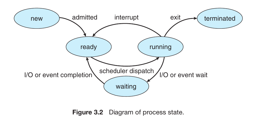
The Process Life Cycle (Process States)
Once a program is loaded into the layout above, it begins its “life.” As it executes, it moves through different States. Think of this as the life cycle of a task:
State
Description
New
The process is currently being created.
Ready
The process is loaded in memory and waiting for the CPU to become available.
Running
Instructions are currently being executed by the CPU.
Waiting
The process is idle, waiting for an event (like user input or a file to load).
Terminated
The process has finished its execution and is being removed from memory.
Fig.3
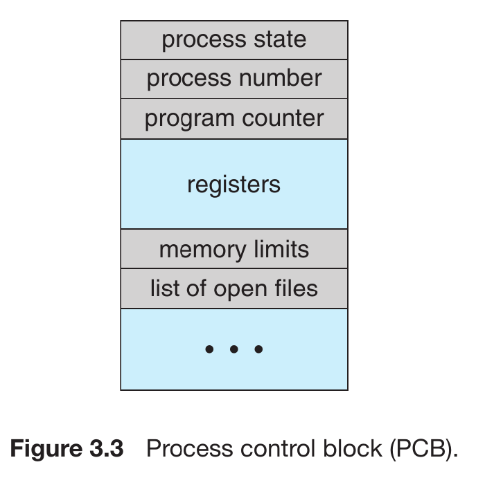
Process Control Block (PCB)
A Process Control Block (PCB), also known as a Task Control Block, is a data structure used by the Operating System to store all the information about a specific process. Think of it as an Identity Card for every running program.
Imagine you are playing a video game and decide to Pause it to do something else. When you return and resume, the game starts exactly where you left off. The computer had to “remember” several things to make this happen:
Your current score.
Your character’s exact location.
The remaining time on the clock.
Your current inventory.
Components of a PCB:
Process State: Indicates the current condition of the process (e.g., New, Ready, Running, Waiting, or Terminated).
Program Counter: Stores the address of the next instruction to be executed for this process.
CPU Registers: These include accumulators, index registers, stack pointers, and general-purpose registers. When a process is interrupted, this state must be saved so it can resume correctly later.
CPU-Scheduling Information: Includes the process Priority, pointers to scheduling queues, and other scheduling parameters.
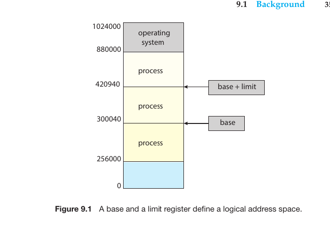
Memory-Management Information: Contains information like the value of base and limit registers, page tables, or segment tables, depending on the memory system used by the OS.
Accounting Information: Includes the amount of CPU and real time used, time limits, account numbers, and job or process numbers.
I/O Status Information: Includes the list of I/O devices allocated to the process, a list of open files, and so on.
Fig.4
What is Thread
is the smallest, basic unit of CPU execution within an operating system, often called a “lightweight process”.
Example: The Multi-threaded MS Word Thread 1: Listens for your keyboard input and displays text on the screen. Thread 2: Runs in the background to check for spelling and grammar errors. Thread 3: Periodically auto-saves your document to the hard drive.
Process scheduling
is an operating system function that manages the execution of processes by selecting a process from the ready queue to run on the CPU, aiming to maximize CPU utilization, throughput, and fairness because we know a CPU core can only run one process at a time.
The CPU core is like a super-fast chef, and the scheduler is like the manager who decides which customer gets served and for how long using priority.
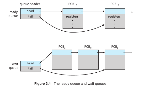
Ready Queue and Wait Queues when many processes are coming
If there are more processes than cores(You have 4 cores and 10 process), excess processes will have to wait until a core is free and can be rescheduled.
Fig.5
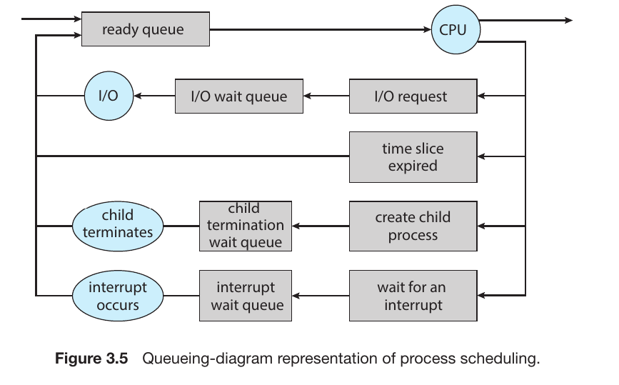
Process scheduling Diagram (Queueing Diagram)
Fig.6
The Starting Point: Ready Queue
Every process begins its journey in the Ready Queue. From here, the Scheduler selects a process and sends it to the CPU to be executed. This specific act of moving a process into the CPU is called Dispatching.
While in the CPU: Four Possible Scenarios
Once a process is running in the CPU, it doesn’t always stay there until it finishes. One of the following four events can trigger its removal:
I/O Request: If the process needs to perform an input or output operation (like saving a file or waiting for a mouse click), it leaves the CPU and enters an I/O Wait Queue. Once the I/O task is completed, it returns to the Ready Queue.
Time Slice Expired: In a Time Sharing system, each process is given a tiny window of time (a Time Slice or Quantum). If the time runs out before the process is done, the OS forcibly removes it and places it at the back of the Ready Queue.
Child Process Creation: If a process creates a new sub-process (Forking a Child), the parent process may move to a Wait Queue until the child process finishes its execution.
Interrupt: If an urgent signal arrives (such as a hardware error or a higher-priority task), the current process is interrupted and moved to an Interrupt Wait Queue so the system can handle the emergency.
The duty of CPU scheduler
I/O-bound Process:
These processes spend most of their time waiting for input/output operations (like reading a file or waiting for a user to click).
They use the CPU only for very short bursts and quickly move back to a Wait Queue.
CPU-bound Process:
These processes perform heavy computations (like video rendering or complex math).
They want to stay in the CPU for as long as possible.
Scheduler’s Strategy: To prevent the system from “hanging” or becoming unresponsivly, the scheduler uses Preemption. It forcibly removes these processes after their time slice expires to give others a chance to run.
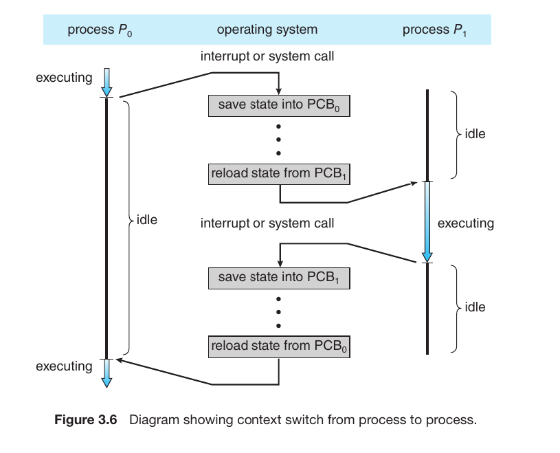
A Context Switch
A Context Switch occurs when the CPU stops executing one process and starts executing another. To ensure the first process can resume exactly where it left off, the OS must save its current “Context” (its state).
How It Works (The Steps)
Using processes $P_0$ and $P_1$ from your diagram as an example:
Interrupt or System Call: While the CPU is running $P_0$, an interrupt or system call occurs, signaling that it’s time to switch.
Save State into $PCB_0$: The OS immediately saves the current state of $P_0$ (register values, program counter, etc.) into its specific $PCB_0$. This is called a State Save.
Idle Time (Overhead): During the switch, the CPU isn’t running any user applications; it is performing OS house-keeping. This time is considered “pure overhead.”
Reload State from $PCB_1$: The OS then fetches the saved state of the next process, $P_1$, from its $PCB_1$. This is called a State Restore.
Execute $P_1$: The CPU now begins running $P_1$ from the point where it was last interrupted.
Fig.7
Essential Facts about Context Switching
Pure Overhead: During a context switch, the CPU does no “useful” work (like playing your music or calculating a formula). It is strictly moving data around. Therefore, the OS tries to make this as fast as possible.
Hardware Dependent: The speed of a context switch depends heavily on the hardware (memory speed, number of registers). Modern processors are so fast that we don’t notice these thousands of switches per second.
The Necessity of Multitasking: Despite the time wasted (overhead), multitasking would be impossible without it.
Mobile Multitasking:
Mobile operating systems like Android and iOS are masters of efficiency. While they offer multitasking similar to computers, they use aggressive strategies to preserve battery life and manage limited RAM.
1. Foreground vs. Background
Mobile systems prioritize what the user is currently looking at to ensure a smooth experience:
Foreground: The app currently visible on your screen. It receives maximum CPU power and memory priority.
Background: When you switch to another app, the previous one moves to the background. To save battery, the system severely limits its activities.
2. App Suspending
Instead of letting every background app run freely, the system often suspends them.
The OS takes a “snapshot” of the app’s current state and keeps it in RAM but stops its execution.
When you return to the app, it resumes instantly from that snapshot, making it feel like it was running the whole time.
3. Background Services
Certain apps are granted “special permission” to remain active even when not on the screen.
Music Players: So your music doesn’t stop when you open Facebook.
Downloads: Allowing a browser to finish a file download in the back.
Notifications: Apps like WhatsApp or Messenger use background tasks to check for new messages.
Terminology: Android calls these Services, while iOS refers to them as Background Tasks.
4. Memory Management (Process Reclamation)
When you open too many apps and the RAM fills up, the OS performs Process Reclamation. It automatically kills the oldest or least-used background process to free up space for the foreground app, preventing the phone from lagging.
5. Split-Screen Multitasking
Modern large-screen phones support True Multitasking via split-screen modes. In this case, two apps act as “Foreground” processes simultaneously, sharing the CPU’s time and screen real estate.
How processes are born and organized into a Process Hierarchy
1. The Process Tree
A process can spawn several new processes during its execution.
Parent Process: The original process that creates others.
Child Process: The new process created by the parent.
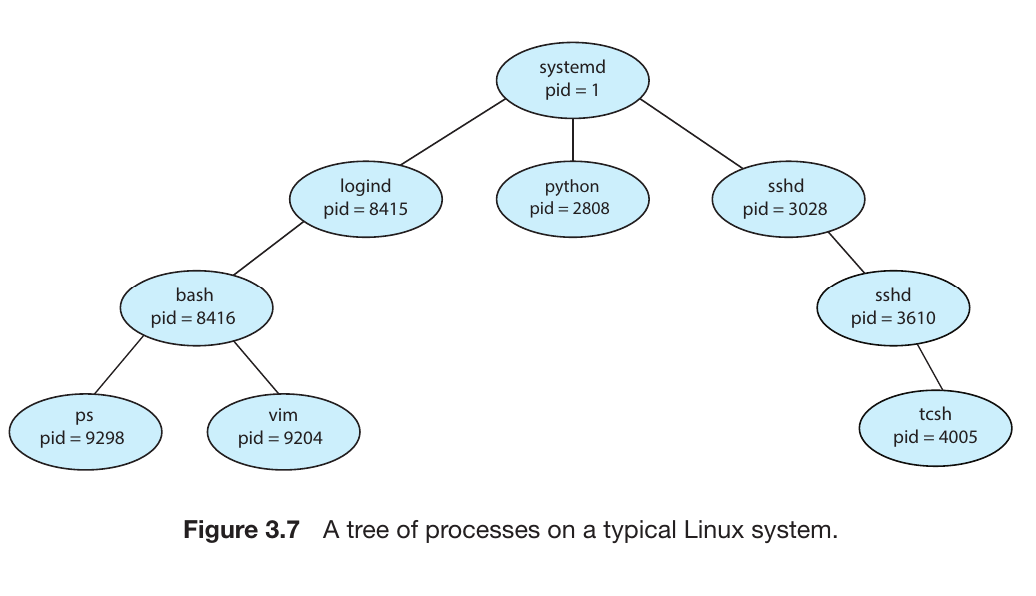
This relationship creates a branching structure known as a Process Tree.
Process Identifier (pid)
To keep track of thousands of processes, the Operating System assigns a unique numerical ID to each one, called the pid. It acts like a student’s ID or a roll number.
In your image, systemd has pid = 1. This is the “root” or “ancestor” of all user processes in a Linux system, created as soon as the computer boots up.
Example: Linux Process Tree
The diagram shows a real-world hierarchy:
systemd (pid 1): The grand-parent of everything.
It spawns logind (manages user logins) and sshd (handles remote connections).
From logind, a bash (command line) process is created, which might then run applications like the vim editor or the ps command.
Creation and Termination
When a parent creates a child, the OS must allocate resources (memory, files, CPU time) for that child.
Creation: The child might share resources with the parent or get its own completely new set.
Termination: Once the child finishes its task, it sends a signal to the OS. The OS then reclaims those resources and removes the process from memory.
Fig.8
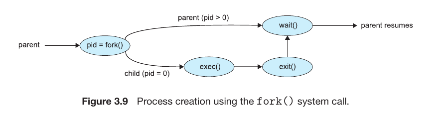
Process create
Linux:fork() (Creates a clone) $\rightarrow$ exec() (Assigns the new task).
Also abdroid used linus architecture so it used fork() for creating process
Windows:CreateProcess() (Starts a new task directly).
Fig.9
Your notes provide an excellent breakdown of how Android handles process creation and memory management. Here is the English translation and technical summary of the Android Process Lifecycle:
1. The Foundation of Process Creation (Zygote)
Since Android is based on the Linux Kernel, it uses the Linux method of process creation but with a specialized twist called Zygote.
Zygote Process: When the Android system boots up, a special parent process named “Zygote” is created. It is the “father” of all Android application processes.
Forking: When you tap an app icon, the system doesn’t start the app from scratch. Instead, it tells the Zygote process to fork(). Zygote creates a clone of itself to launch the new app process. This makes app startup incredibly fast because the clone already has the core Android libraries pre-loaded.
Android Process Hierarchy (Importance Levels)
The “life expectancy” of a process is determined by its importance. When the system runs low on memory (RAM), it uses this hierarchy to decide which process to kill first:
The 5 Levels of Importance:
Foreground Process (Highest Priority):
The app you are currently interacting with on the screen.
The system will never kill this process unless the memory is so low that even the OS itself is about to crash.
Visible Process:
An app that is not in the focus but is still visible to you.
Example: A transparent pop-up or a small window overlapping another app.
Service Process:
Apps that aren’t on the screen but are performing essential tasks in the background.
Example: Playing music in the background or a file being downloaded.
Background Process:
Apps that were recently used but are now minimized (e.g., you were on Facebook but switched to WhatsApp).
Android will kill these first if more memory is needed for a foreground app.
Empty Process (Lowest Priority):
These processes are not doing any active work. They stay in RAM simply as a “cache” so the app opens instantly if you click it again.
Android clears these immediately whenever memory is needed.
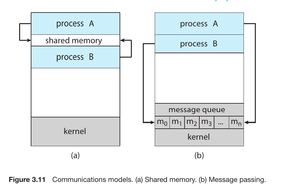
is a mechanism that allows processes to communicate and share data with each other while they are running.There are two method of IPC,
shared memory
Message passing.
A) Shared Memory
Processes agree on a specific region of memory that they can both read from and write to.
Advantage: It is extremely fast because data doesn’t have to be moved; it’s already there.
Disadvantage: It is harder to manage. If both processes try to write at the exact same time, it causes a Conflict (Race Condition). The programmer must handle the synchronization.Also contains producer and consumer problem
B) Message Passing
Processes communicate by sending and receiving small packets of data (messages) through the OS Kernel.
Advantage: It is easier to implement and much safer for Distributed Systems (e.g., two different computers talking over a network). No conflicts occur because the Kernel acts as the postman.
Disadvantage: It is slower than shared memory because every message must go through the Kernel, adding “overhead.”
Fig.10
There are three techinuqe for Message passing
1. Naming: How Processes Identify Each Other
Direct Communication:
Symmetry: Both processes must explicitly name each other. For example, send(P, message) sends to process P, and receive(Q, message) receives specifically from process Q.
Asymmetry: The sender names the recipient, but the recipient doesn’t know the sender beforehand. The recipient uses receive(id, message), and the variable id is filled with the sender’s name once the message arrives.
Indirect Communication:
Processes communicate via Mailboxes or Ports.
Think of this like a public drop-box: Process A puts a message in Mailbox 1, and Process B retrieves it. This allows multiple processes to communicate through a single shared link.
2. Synchronization: Blocking vs. Non-blocking
This determines whether a process pauses its execution during communication. This is often referred to as Synchronous vs. Asynchronous communication:
Blocking Send: The sender is “blocked” (stops working) until the message is received by the recipient or the mailbox.
Non-blocking Send: The sender sends the message and immediately resumes its other tasks without waiting.
Blocking Receive: The receiver stops and waits until a message is actually available.
Non-blocking Receive: The receiver checks for a message; if there is one, it takes it; if not, it continues working instead of waiting.
3. Buffering: Managing the Message Queue
When messages are in transit, they reside in a temporary queue. The capacity of this queue dictates how the processes behave:
Zero Capacity: The queue has a length of 0. The sender must wait until the receiver is ready to take the message. This direct hand-off is called a Rendezvous.
Bounded Capacity: The queue has a fixed length ($n$). The sender can keep sending until the queue is full; once full, the sender must wait.
Unbounded Capacity: The queue is theoretically infinite. The sender never has to wait, as there is always room to “drop off” the message.
4. Real-World Analogy: The Chat App
Indirect Communication: A Group Chat. Everyone sends messages to a central Group ID (Mailbox), and any member can read them.
Blocking Send: Imagine a “Walkie-Talkie” or an app that shows a loading spinner saying “Sending…” and prevents you from doing anything else until the message is delivered.
Non-blocking Send: A typical SMS or WhatsApp message. You hit send and immediately go back to scrolling your feed while the message sends in the background.
Example for IPC
In windows
What is ALPC?
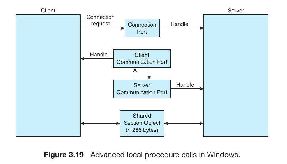
In the Windows operating system, when two processes on the same computer (e.g., a user application and a system service) need to communicate, they use ALPC. It is a high-speed, localized version of the standard RPC (Remote Procedure Call), specifically optimized for internal system communication.
Fig.11
2. How It Works (The Port Mechanism)
ALPC establishes communication using Port Objects, :
Connection Port: The server process creates and publishes a connection port. When a client wants to communicate, it sends a connection request to this port.
Communication Ports: Once the server accepts the request, the OS creates a pair of dedicated ports—a Client Communication Port and a Server Communication Port—to handle the actual message exchange.
3. Three Techniques for Message Delivery
ALPC is “smart”—it chooses the delivery method based on the size of the data:
Small Messages (Up to 256 bytes): The message is copied directly into the port’s queue. This is extremely fast for simple commands.
Medium Messages: If the message is larger than 256 bytes, a Section Object (Shared Memory) is used. The sender places the data in the shared section, and the receiver gets a pointer (address) to that data.
Large Data: For massive data transfers, a specialized API allows the server to read from or write directly into the client’s address space without extra copying.
4. Why is ALPC Unique?
ALPC is a “hybrid” model. It uses Message Passing for small tasks to maintain security and simplicity, but switches to Shared Memory for large tasks to maintain high speed. It gives Windows the best of both worlds.
What are Pipes?
A pipe acts as a conduit or a “tunnel” that allows data to flow from one process to another. When designing or implementing a pipe, four key factors must be considered:
Direction: Is the communication unidirectional (one-way) or bidirectional (two-way)?
Duplex: If it is bidirectional, is it Half-duplex (one direction at a time) or Full-duplex (both directions simultaneously)?
Relationship: Is a relationship (like Parent–Child) required between the communicating processes?
Network: Does the pipe work only on the local machine, or can it communicate over a network?
2. Ordinary Pipes
Ordinary pipes follow a strict Producer-Consumer pattern.
Mechanism: The Producer writes data to the “write end” of the pipe, and the Consumer reads it from the “read end.”
Direction: These are typically unidirectional. If two-way communication is needed, two separate pipes must be created.
Relationship: In Unix-based systems, these require a Parent-Child relationship. The pipe is created by a parent, which then spawns a child process to share the communication link.
3. Named Pipes
Named pipes are significantly more robust and flexible than ordinary pipes.
Bidirectional: They support two-way communication.
No Relationship Required: Processes do not need to be related (no Parent-Child requirement). Any process that knows the name of the pipe can use it to communicate.
Persistence: While ordinary pipes vanish once the processes finish, a Named Pipe exists as a file in the system until it is explicitly deleted. In Unix, these are often called FIFOs (First-In, First-Out).
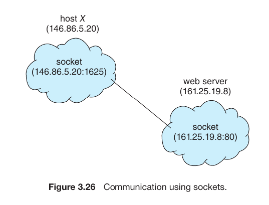
What is a Socket?
A Socket is defined as an endpoint for communication between two processes over a network. When two computers (e.g., your laptop and a web server) communicate, each computer uses a socket to send and receive data.
2. How is a Socket Formed?
A socket is a combination of two critical identifiers:
IP Address: The unique address of the computer on the network.
Port Number: A specific “door” or “channel” on that computer assigned to a particular application.
Example If Host X has the IP address 146.86.5.20 and wants to communicate with a server, its unique socket might be 146.86.5.20:1625. The :1625 is the port number assigned to the specific app on Host X.
Fig.12
3. Well-known Ports
Servers usually “listen” on standard ports so that clients know exactly where to find them:
Port 80: Web Servers (HTTP).
Port 21: File Transfer (FTP).
Port 22: Secure Login (SSH).
Ports below 1024 are considered Well-known Ports, reserved for standard system services.
4. Types of Sockets in Java
Your text mentions three ways Java handles network communication:
Connection-oriented (TCP): Implemented via the Socket class. It ensures 100% data delivery (reliable).
Connectionless (UDP): Implemented via the DatagramSocket class. It is faster but doesn’t guarantee the data will arrive (unreliable).
MulticastSocket: Used to send a single message to multiple subscribers simultaneously.
Why do processes need to talk?
By default, processes are isolated for security—one process cannot see another’s data. However, communication is necessary for:
Information Sharing: Copying text from a website and pasting it into a Word document requires data to move between two independent processes.
Computation Speedup: A massive task can be split into smaller pieces, with multiple processes working on them simultaneously to save time.
Modularity: Breaking a complex system into smaller, manageable parts that work together.
Multi-process Architecture: The Google Chrome Example
Google Chrome is famous for its “heavy” memory usage, but this is a deliberate design choice for stability and security:
Process Isolation: Chrome creates a separate Renderer Process for every single tab you open.
Stability: If one website crashes or hangs, it only affects that specific tab. The rest of your browser and other tabs stay open.
Security (Sandboxing): Because each tab is a separate process, a malicious website is trapped in a “Sandbox.” It cannot easily jump out of its process to steal files from your computer.
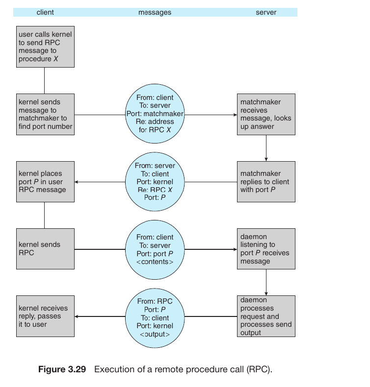
The Mechanism of RPC (Remote Procedure Call)
RPC is a technology that allows you to execute a function on a remote server as if it were a local function on your own computer. This process involves 5 key steps:
Fig.13
Client-side Call: The user calls a function. Instead of running locally, this call is intercepted by a Client Stub (a proxy).
Marshaling (Packing): The Client Stub packs the function name and its arguments into a standardized message format. This process is called Marshaling. It then hands this package to the local Kernel.
Network Transmission: The Client’s Kernel transmits the message over the network to the Server.
Unmarshaling (Unpacking): The Server’s Kernel receives the message and passes it to the Server Stub. The stub unpacks the data (Unmarshaling) to understand which local function needs to be triggered.
Execution & Result: The Server executes the task and sends the result back through the same path in reverse (Server Stub $\rightarrow$ Kernel $\rightarrow$ Network $\rightarrow$ Client).
Why is RPC Important?
Transparency: For a programmer, the complexity of the network is hidden. You feel like you are working on your own machine, even if the actual heavy lifting is happening on a supercomputer miles away.
XDR (External Data Representation): Different computers (like a Mac and a Windows PC) might store data differently. RPC uses XDR to convert data into a universal format so that both sides can understand each other.
Android RPC and the Binder Framework
The text explains how Android manages communication between different applications and system services. While traditional RPC connects a client and server over a network, Android uses it to bridge the gap between separate processes on the same phone.
1. IPC (Inter-Process Communication) In Android, every app runs in its own isolated process for security. To share data or request a task from another app (or the system), Android uses RPC as a form of IPC.
2. The Binder Framework The Binder is the heart of Android’s communication system. It is a specialized framework that allows one process to call a routine in another process’s address space as if it were a local call. It acts as the “messenger” that carries requests and data between apps.
3. Application Components Android apps are built from various components (like Activities, Services, and Content Providers). These components often need to talk to each other or to system components. The RPC/Binder mechanism ensures these interactions are seamless and secure.
Real-World Example
Imagine you are using a Food Delivery App. When you click to “Pay,” the delivery app needs to communicate with a Payment App (like PayPal or a Bank app) installed on your phone.
The Food App doesn’t have access to your bank details.
Instead, it uses RPC/Binder to send a request to the Payment App.
The Payment App processes the request and sends a “Success” message back.
A thread
is a small part of a process or program that can run independently. It is sometimes called a “lightweight process”.
A thread is the smallest unit of CPU utilization. Each thread possesses its own:
Thread ID: A unique identifier.
Program Counter (PC): Tracks which instruction to execute next.
Register Set: Stores current working data.
Stack: Manages function calls and local variables.
Fig.14
Thread vs process
The Process (Chrome.exe)
When you open Chrome, the operating system starts one or more Processes.
Example: Imagine you have three tabs open: Facebook, YouTube, and Gmail.
In modern Chrome, each of these tabs usually runs as a separate process (independent chrome.exe that you see in task manager).
Why? (Process Isolation): If the Facebook tab encounters a heavy script and crashes, your YouTube and Gmail tabs stay alive. Because they are separate processes, they don’t share the same memory “safety bubble.”
The Thread - The “Workers”
Now, look inside a single tab, like the YouTube tab. That one process needs to do many things at once. These smaller units of work are Threads or Myltitherad.
Thread 1: Responsible for streaming and rendering the video.
Thread 2: Loading and updating the comment section.
Thread 3: Listening for your mouse clicks or keyboard inputs.
Collaboration: All these threads work inside the YouTube process and share the same memory (RAM) allocat
Multithreaded Server Architecture
Request: A client sends a request to the server for a specific service or piece of data (e.g., clicking a link on a website).
Create New Thread: Instead of the main server process doing the work itself, it spawns a new thread specifically to handle that client’s request.
Resume Listening: Once the new thread takes over the task, the main server process goes back to “listening” for the next client. It doesn’t wait for the first task to finish.
Fig.14
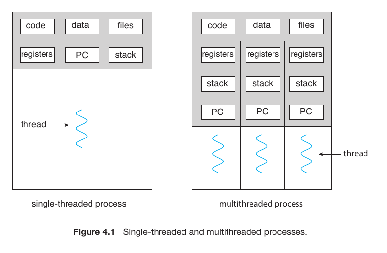
Comparing Single-threaded vs. Multithreaded Processes
Single-threaded Process: Has only one set of Registers, Stack, and PC. It is a “serial” worker—it must finish Task A before starting Task B.
Multithreaded Process: Features multiple threads. Notice how they all sit under the same Code/Data/Files umbrella but have their own Registers and Stacks. This allows the process to execute multiple parts of its code across different CPU cores at the exact same time.
4 Main Benefits of Multithreading:
1. Responsiveness
Multithreading allows an application to stay interactive even if one part of it is busy or blocked.
Simple Example: In a photo editing app, one thread can save a heavy image to the disk while another thread allows you to keep clicking buttons. The app doesn’t “freeze” or show “Not Responding.”
2. Resource Sharing
Processes are isolated, but threads are social. They share the memory and resources of the process they belong to by default.
Simple Example: Because they share the same data space, different threads can work on the same file or variable without needing complex communication tools like “Shared Memory.”
3. Economy (Cost-Effective)
Creating a new process is “expensive” for the computer—it takes a lot of time and memory to set up.
Simple Example: Creating a thread is much faster and “cheaper” because it reuses what is already there. Switching between two threads (Context Switch) is also much faster for the CPU than switching between two processes.
4. Scalability
This is where you get the most out of modern hardware.
The Difference: A single-threaded app can only use one CPU core, no matter how powerful your PC is. A multithreaded app can spread its threads across multiple cores, running them truly at the same time (Parallelism).
Multicore programming
involves designing software to run on processors with two or more cores, enabling true parallel execution to boost performance beyond single-core limitations.
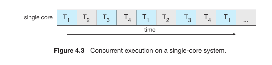
Concurrency (Single-Core Systems)
In a system with only one CPU core, the processor can only do one thing at a time.Doing many things at once by switching between threads extremely fast.
Mechanism: This is called Interleaved Execution. The CPU works on $T_1$ for a tiny fraction of a second, then switches to $T_2$, then $T_3$, and so on.
Result: It looks like the tasks are happening simultaneously, but they are actually just taking turns very quickly.
Fig.14
Parallelism (Multi-Core Systems)
Parallelism occurs when a system has two or more CPU cores. Each core can handle its own separate thread independently.
Mechanism: This is Simultaneous Execution. For example, Core 1 executes $T_1$ while Core 2 executes $T_2$ at the exact same instant in time.
Result: The system is actually performing multiple tasks at the same time, leading to a massive boost in speed.
Programming Challenges for Multicore Systems
To exploit the power of multiple cores, programmers can’t just write “normal” code; they must think in parallel. This presents five major challenges (the first two are covered here):
Identifying Tasks: Programmers must examine applications to find areas that can be divided into separate, concurrent tasks. These tasks should ideally be independent of one another.
Balance: It is crucial to ensure that the divided tasks perform equal work. If one core is overloaded while another core sits idle, the efficiency of the multicore system is wasted.
Data Splitting: Just as tasks are divided, the data itself must be partitioned to run on different cores. If the data isn’t split correctly, threads will end up waiting for each other, wasting the multicore advantage.
Data Dependency: This is a major hurdle. When Task A needs the result of Task B to continue, they are “dependent.” Programmers must ensure synchronization so that threads don’t use “stale” or incorrect data.
Testing and Debugging: This is notoriously difficult. In a single-threaded app, the execution path is a straight line. In multithreaded apps, there are many paths running at once. Errors might only happen sometimes (Race Conditions), making them very hard to recreate and fix.
Amdahl’s Law
Amdahl’s Law is a mathematical formula used to predict the maximum theoretical speedup of an application when using multiple processors.
The Core Logic:
Every application has two parts:
Serial (S): Portions that must be done one after another (cannot be parallelized).
Parallel (1 - S): Portions that can be split across multiple cores.
$S$: The portion of the application that must be performed serially.
$N$: The number of processing cores.
Why This Matters (The “Law of Diminishing Returns”)
As you correctly noted:
If 25% of your app is serial ($S = 0.25$), even if you add infinite cores ($N$), your speedup will never exceed 4x.
This teaches us that the serial component of the software has a disproportionate impact on the overall speed, regardless of how powerful the hardware is.
Types of Parallelism for multicore system
To maximize the speed of a multicore system, work is divided in two primary ways:
Data Parallelism (Same Task, Different Data)
This approach focuses on distributing subsets of the same data across multiple computing cores and performing the same operation on each core.
Visual Analysis: A large dataset is split into four blocks. Cores $core_0$ through $core_3$ work simultaneously on these separate blocks, but they are all running the exact same instruction.
Real-world Example: If you need to brighten 1,000 photos, you give 250 photos to each of the 4 cores. Every core is doing the same task (brightening), just on different files.
This approach focuses on distributing different tasks (threads) across multiple cores. Each core performs a unique operation.
Visual Analysis: The threads are distinct. $core_0, core_1, core_2,$ and $core_3$ are each executing a different piece of code or service.
Real-world Example: In a video editing suite:
Core 0: Renders the video frames.
Core 1: Processes the audio track.
Core 2: Handles the user interface and mouse clicks.
Core 3: Performs background auto-saving.
Multithreading Models
To understand how threads work, we must distinguish between the two “layers”:
User Threads: Managed by thread libraries at the user level, without direct kernel intervention.
Kernel Threads: Managed directly by the Operating System.
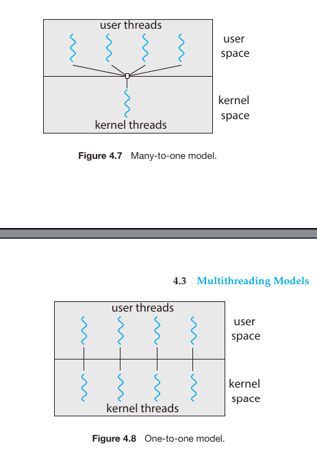
Many-to-One Model
In this model, many user-level threads are mapped to a single kernel thread.
Key Characteristics for many to one model
Efficiency: Thread management is done in “User Space” by a library. This is very fast because it doesn’t require “Context Switching” into the kernel to create or manage threads.
The Blocking Problem: This is the model’s biggest weakness. Because there is only one connection to the kernel, if one user thread makes a “blocking” call (like waiting for a file to load), the entire process stops. The kernel sees only one thread, and that thread is now stuck.
No True Parallelism: Even if you have a 16-core CPU, the Many-to-One model cannot run threads in parallel. Since the kernel only sees one thread, it can only schedule that one thread on one core at a time.
Fig.14
Your summary of the three multithreading models perfectly highlights the trade-offs between concurrency, complexity, and performance. It is fascinating to see how the “best” theoretical model (Many-to-Many) lost out to the “simplest” robust model (One-to-One) due to modern hardware power.
Here is the English explanation of these advanced multithreading models:
1. One-to-One Model
In this model, every single User Thread is mapped to its own dedicated Kernel Thread.
The Big Win: It solves the “blocking” problem of the Many-to-One model. If one thread waits for a file to download, the other threads can keep running because they have their own independent paths to the Kernel.
Parallelism: This is the best model for multicore processors, as the OS can put different threads on different cores simultaneously.
The Catch: Creating a kernel thread for every user thread has an “overhead” cost. However, Windows and Linux use this model because modern PCs are now powerful enough to handle thousands of kernel threads easily.
2. Many-to-Many Model
This model multiplexes many user-level threads to a smaller or equal number of kernel threads.
Flexibility: Developers can create as many user threads as they want, and the Kernel manages a “pool” of kernel threads to handle them.
Efficiency: It doesn’t overwhelm the system with too many kernel threads, yet it still allows multiple threads to run in parallel.
The Reality Check: While it sounds perfect on paper, it is extremely difficult to code into an Operating System. Managing the “mapping” between layers is complex and often slower than just using One-to-One.
3. Two-level Model
This is a hybrid approach. It mostly follows the Many-to-Many logic but allows a specific, high-priority user thread to be “bound” to a single dedicated kernel thread.
Why use it? If you have a critical task (like a real-time audio stream) that must never be delayed by other threads, you “bind” it to its own kernel thread while the rest of the app uses the Many-to-Many pool.
Thread Libraries
A thread library provides the API (Application Programming Interface) that programmers use to create and manage threads. There are two main ways these libraries are implemented:
User-space library: All code and data structures for the library exist in user space. Invoking a function in the library results in a local function call, not a system call.
Kernel-level library: Supported directly by the OS. The library code exists in kernel space, and calling an API function typically results in a system call to the kernel.
The “Big Three” Libraries:
POSIX Pthreads: A POSIX standard ($IEEE$ $1003.1c$) defining an API for thread creation and synchronization. It is a specification, not an implementation, commonly used on UNIX-based systems (Linux, Solaris, macOS).
Windows Threads: A kernel-level library available on Windows systems.
Java Threads: Since Java is platform-independent, its threading API is managed by the JVM. It typically maps to whatever native thread library is available on the host OS (Windows or Pthreads).
2. Strategies for Threading
When designing multithreaded programs, developers choose between two main strategies depending on whether the parent thread needs to wait for its children:
Asynchronous Threading
The Concept: Once the parent creates a child thread, the parent resumes its execution. The parent and child operate independently.
Analogy: “You do your work, I’ll do mine.”
Best For: Event-driven systems, responsive User Interfaces (UI), and Web Servers. Since the threads are independent, there is usually little data sharing between them.
Synchronous Threading
The Concept: The parent thread creates one or more children and then must wait for all of them to terminate before it resumes. This is often called the “Fork-Join” model.
Analogy: “Finish your part of the task, then we will combine our results to move forward.”
Best For: Heavy data processing or mathematical calculations. For example, if you are summing a massive array, you split it into four parts for four threads. The parent waits for the four partial sums to return so it can calculate the final total.
Thread Pools and their role in Android:
The Problem with “On-Demand” Threading
As you correctly noted, creating a new thread for every task (like a web request) leads to two major issues:
Time Latency: Spawning a thread takes a few milliseconds. In high-speed web services, these milliseconds add up.
Resource Exhaustion: If a server gets 10,000 requests at once and tries to create 10,000 threads, the system’s RAM and CPU will likely crash due to “thrashing.”
The Solution: Thread Pools
A Thread Pool is a collection of pre-instantiated, “standby” threads.
Process: When a task arrives, it is placed in a Work Queue. If a thread in the pool is available (idle), it picks up the task.
Reusability: Once the task is finished, the thread returns to the pool and waits for the next assignment. It is never “deleted.”
Overflow: If all threads are busy, the task simply waits in the queue until a worker becomes free.
Key Benefits of the Pool Model
Lower Latency: Since threads already exist, the task starts executing immediately.
System Stability (Bound Resources): By limiting the maximum number of threads (e.g., matching the number of CPU cores), you ensure the server never takes on more work than it can physically handle.
Task Management: It allows for different strategies, such as running a task after a certain delay or executing it periodically.
Android and Thread Pools
In Android, keeping the UI Thread (Main Thread) free is critical. If you perform a heavy task on the UI thread, the app freezes.
RPC & AIDL: When your app communicates with other apps or system services via Remote Procedure Calls (RPC), Android uses a thread pool to handle those requests in the background.
Concurrency: This ensures that if multiple background services are asking for data at once, the system doesn’t bog down—it manages them through a controlled pool of threads.
Java Thread Pool Models
In Java, you don’t create threads manually using new Thread() for every task. Instead, you use the Executor Framework. The Executors class provides factory methods to create different types of pools:
1. Single Thread Executor
Concept: Creates a pool with exactly one worker thread.
Behavior: It processes tasks one by one in a strictly sequential order. If the thread dies due to a failure, a new one is created to take its place.
Code:Executors.newSingleThreadExecutor()
Best For: Tasks that must be executed in a specific order without overlapping.
2. Fixed Thread Executor
Concept: Creates a pool with a fixed number of threads (defined by the programmer).
Behavior: If all threads are busy, new tasks wait in a queue (LinkedBlockingQueue) until a thread becomes free.
Code:Executors.newFixedThreadPool(int nThreads)
Best For: Servers with predictable loads where you want to limit resource usage.
3. Cached Thread Executor
Concept: Creates a pool that creates new threads as needed but reuses previously constructed threads when they are available.
Behavior: It is “unbounded.” If a thread is idle for 60 seconds, it is terminated and removed from the cache.
Code:Executors.newCachedThreadPool()
Best For: Short-lived asynchronous tasks where the volume of tasks varies frequently.
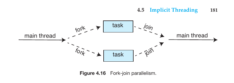
What is the Fork-Join Model?
The Fork-Join model is a process where a large task is divided into smaller sub-tasks and executed simultaneously (parallelly) using multiple threads. It primarily operates in two stages:
Fork: When a main thread or parent thread divides its work into one or more smaller sub-tasks (child tasks), it is called a ‘Fork’. As shown in diagrams, this is the point where two or more separate tasks branch out from a single main thread.
Join: Once the smaller sub-tasks complete their execution, the parent thread collects those results and merges them back into a single, unified thread. This step is known as a ‘Join’.
Fig.15
What is OpenMP?
OpenMP is an API (Application Programming Interface) used for Parallel Programming in C, C++, and FORTRAN programming languages. It primarily functions within a ‘Shared-Memory’ environment.
How does it work?
It utilizes Compiler Directives. When a developer wants a specific section of code to run simultaneously (parallelly), they add special directives to that section.
Parallel Regions: The segments of code that can run on multiple processors at the same time are called ‘Parallel Regions’.
Automation: The OpenMP run-time library automatically divides these regions into multiple threads for execution.
Grand Central Dispatch (GCD)
This is a technology developed by Apple to simplify parallel programming on macOS and iOS. Its core concept is that the developer does not need to worry about managing threads; they only need to define the tasks.
Key Features:
Dispatch Queue: GCD organizes tasks into a queue or line. From here, tasks are dispatched to a Thread Pool.
Serial Queue: Tasks are completed one by one (FIFO - First In First Out). A new task does not start until the previous one is finished. These are also called Main Queues or Private Queues.
Concurrent Queue: Tasks still leave the queue in FIFO order, but multiple tasks can start and run at the same time (Parallel execution). These are known as Global Dispatch Queues.
QoS (Quality of Service): Tasks are categorized based on their importance:
User-interactive: Urgent tasks like User Interface (UI) updates or event handling.
User-initiated: Tasks requested by the user that might take a short amount of time.
Intel Thread Building Blocks (TBB)
TBB is a template library for C++. It is primarily used to take full advantage of multi-core processors.
Key Features:
Library-based: It does not require a special compiler; it works as a standard C++ library.
Task Scheduler: TBB itself determines which task goes to which thread. It performs Load Balancing and optimizes cache memory usage.
Parallel Loops: It includes the parallel_for template to parallelize standard for loops.
Here is the English translation of your detailed explanation regarding Multi-threaded Programming Issues and System Calls:
Threading Issues and Challenges
The fork() and exec() System Calls (Section 4.6.1)
These two system calls behave uniquely in a multithreaded environment:
fork(): If one thread in a process calls fork(), does the new process duplicate all threads or only the calling thread?
Version 1: Only the thread that called fork() is duplicated in the child process.
Version 2: All threads from the parent process are duplicated in the child.
exec(): If exec() is called immediately after fork(), duplicating all threads is unnecessary because exec() replaces the entire process image with a new program.
Signal Handling
Signals are used in UNIX systems to notify a process that a particular event has occurred. In multithreading, the challenge is deciding which thread should receive the signal.
Synchronous Signals: Delivered to the specific thread that caused the signal (e.g., division by zero or illegal memory access).
Asynchronous Signals: Generated by external events (e.g., pressing Ctrl+C). These can be delivered to one specific thread, all threads, or a designated signal-handling thread.
Thread Cancellation
This involves terminating a thread before it has completed its task.
Asynchronous Cancellation: One thread terminates the target thread immediately. This is risky as the thread might be holding a resource or updating shared data.
Deferred Cancellation: The target thread periodically checks a flag to see if it should terminate. It shuts itself down only at “cancellation points” where it is safe to do so.
Thread-Local Storage TLS
While threads within a process share data, sometimes a thread needs its own unique copy of certain data. This is TLS. Unlike local variables (which only exist inside a function), TLS data is visible across all functions within that specific thread.
Scheduler Activations
This is a communication mechanism between the User-Thread Library and the Kernel.
It uses an intermediate data structure called LWP (Lightweight Process), which acts like a virtual processor.
Upcalls: If a thread is about to block, the kernel sends an “upcall” to the thread library, allowing the library to schedule another thread so the application doesn’t freeze.
Your explanation of how fork() and exec() operate within a multi-threaded environment is spot on. You’ve captured the core dilemma: resource efficiency versus state duplication.
Here is the English translation of your practical example and analysis:
How fork() and exec() Work in Multi-threaded Programs: A Practical Example
Imagine you have a Web Browser process running. Inside this process, there are three active threads:
Thread A: Managing the User Interface (UI).
Thread B: Downloading a file in the background.
Thread C: Calling fork() to open a new program (e.g., a Calculator).
1. The fork() Scenario
When Thread C calls the fork() system call, the Operating System creates a new ‘Child Process’. The number of threads in this child process depends on the OS implementation:
Duplicate All Threads: If the OS copies every thread, the child process will also have three threads (A, B, and C). This is necessary if the child process is intended to continue the exact same multi-threaded work as the parent.
Duplicate Only Calling Thread: In this case, the child process becomes Single-threaded. It will only contain a copy of Thread C. Threads A and B will not exist in the child.
2. The exec() Integration
Usually, the primary goal of calling fork() is to execute a completely different program. Let’s say Thread C wants to launch a Calculator app.
Step 1: Thread C calls fork(). A child process is created containing only Thread C.
Step 2: The child process immediately calls exec().
Result: As soon as exec() is called, the existing thread (Thread C) in the child process is removed, and the Calculator program’s code is loaded into that memory space.
Why is it unnecessary to copy all threads?
If we had copied Threads A and B during the fork(), they would have been deleted the moment exec() was called anyway. Since exec() replaces the entire process memory with a new program, copying extra threads is a waste of CPU and memory. Therefore, if exec() follows fork(), copying only the calling thread is the most efficient approach.
Technical Comparison: Windows vs. Linux Threads
Windows Threads
Windows follows a one-to-one mapping model, meaning every user-level thread corresponds to a unique kernel thread.
Core Components of a Thread:
Thread ID: A unique identifier for each thread.
Register Set: Represents the current status of the processor.
Program Counter: The memory address of the instruction currently being executed.
Stacks: Windows threads utilize two stacks—a User Stack for user-mode execution and a Kernel Stack for kernel-mode execution.
Primary Data Structures:
The Windows thread architecture is composed of three primary blocks:
ETHREAD (Executive Thread Block): Located in kernel space; it contains the thread’s start address and a pointer to the parent process.
KTHREAD (Kernel Thread Block): Also in kernel space; it contains scheduling and synchronization information.
TEB (Thread Environment Block): Located in user space; it stores the thread identifier, user stack, and Thread-Local Storage (TLS).
Linux Threads
Linux does not make a strict distinction between a “process” and a “thread.” Instead, it refers to them generally as Tasks.
The clone() System Call:
To create threads, Linux frequently uses the clone() system call instead of fork(). Its unique feature is the ability to control exactly how much data is shared between the parent and child tasks via specific flags:
CLONE_VM: Shares the memory space (the defining characteristic of a thread).
CLONE_FS: Shares file system information.
CLONE_SIGHAND: Shares signal handlers.
CLONE_FILES: Shares the list of open files.
The Key Difference:
If clone() is called without any flags, it behaves like a standard fork() (creating a separate process). If flags are set to share resources, it functions as a thread. This flexibility in Linux is the foundational technology for Containers (like Docker).
CPU Scheduling
CPU Scheduling is the foundation of Multiprogrammed Operating Systems. When multiple programs or processes run simultaneously on a computer, the Operating System decides which process will get access to the CPU and when.
The primary goal is to ensure the CPU is never idle (unless there are no processes at all), thereby maximizing the system’s throughput and productivity.
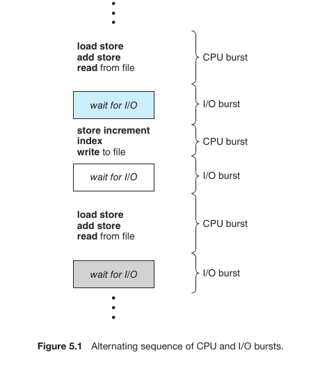
CPU and I/O Bursts (The Process Cycle)
When a process or program runs on a computer, it alternates between two primary states:
CPU Burst: When the processor is executing instructions or performing calculations (e.g., load, store, add).
I/O Burst: When the process is waiting for input or output (e.g., reading from or writing to a file, waiting for user input).
Fig.16
Understanding the Life Cycle
As shown in the diagram, a process moves through these stages in a predictable pattern:
Initial CPU Burst: The process begins by performing calculations. During this time, it actively uses the processor.
Wait for I/O (I/O Burst): Once it needs data from a file or a device, it enters a wait state. During this period, the CPU is free and can be used for other tasks.
Subsequent CPU Burst: After the I/O operation is complete, the process returns to the CPU to continue its next set of instructions (e.g., store, increment, write to file).
Cyclical Process: This continues until the task is finished. This pattern is known as the Alternating sequence of CPU and I/O bursts.
The CPU-I/O Burst Cycle
As a process runs, it functions in a cycle: it uses the CPU for a period (CPU Burst), waits for input/output (I/O Burst), and then returns to the CPU again.
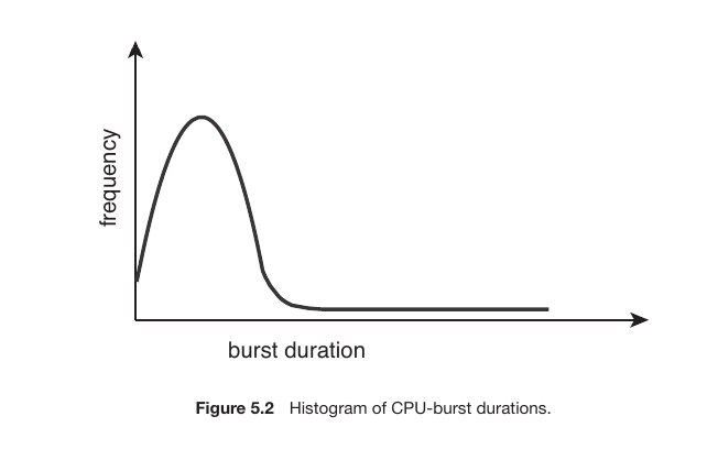
The Histogram provides a crucial insight:
Short CPU Bursts: Most processes have very short CPU bursts. They perform a few quick calculations and then immediately move to an I/O operation. This is represented by the high peak on the left side of the graph.
Long CPU Bursts: Only a few processes require long, continuous CPU time (e.g., complex mathematical simulations). This is represented by the low “tail” on the right side of the graph.
Fig.16
The CPU Scheduler
Whenever the CPU becomes idle, the Operating System must decide which process from the Ready Queue in memory will be allocated to the processor next. This selection process is handled by the CPU Scheduler (also known as the Short-term Scheduler).
Ready Queue: This is where processes wait for their turn. It is not always a simple FIFO (First-In, First-Out) queue; it can be implemented as a Priority Queue, a linked list, or even a tree.
PCB (Process Control Block): The scheduler uses the information stored in each process’s PCB to manage its state and transitions.
1.Preemptive vs. Non-preemptive Scheduling
CPU scheduling decisions are typically made under these four circumstances:
When a process switches from the Running to the Waiting state (e.g., an I/O request).
When a process switches from the Running to the Ready state (e.g., a timer interrupt).
When a process switches from the Waiting to the Ready state (e.g., I/O completion).
When a process Terminates.
The Key Differences:
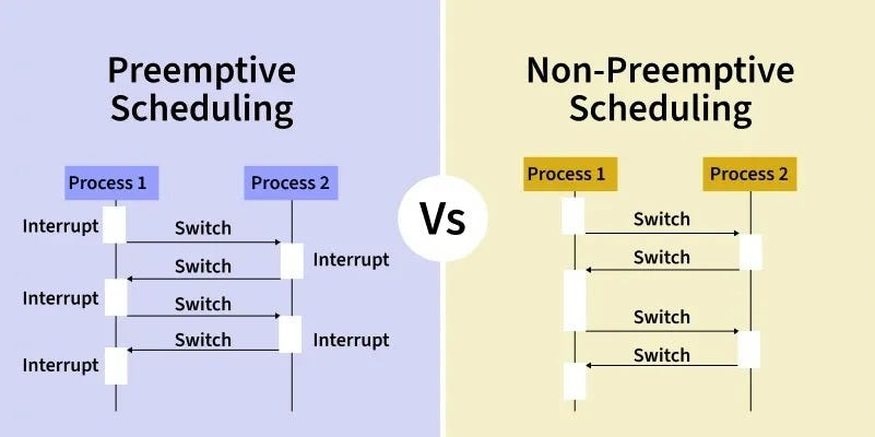
Non-preemptive (Cooperative): Scheduling occurs only under circumstances 1 and 4. Once a process gains control of the CPU, it keeps it until it either finishes or voluntarily releases it to wait for I/O.
Preemptive: Used by all modern operating systems (Windows, macOS, Linux). The OS can forcibly take the CPU away from a running process to give it to another (circumstances 2 and 3).
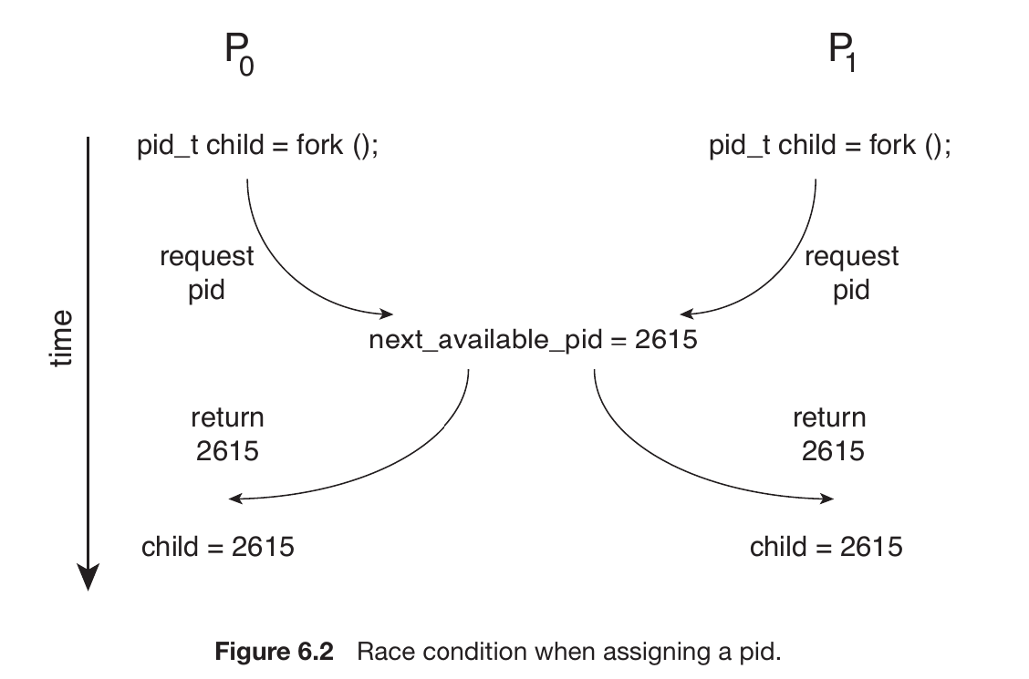
Challenge: Preemptive scheduling can lead to Race Conditions because a process might be interrupted while it is in the middle of updating shared data.
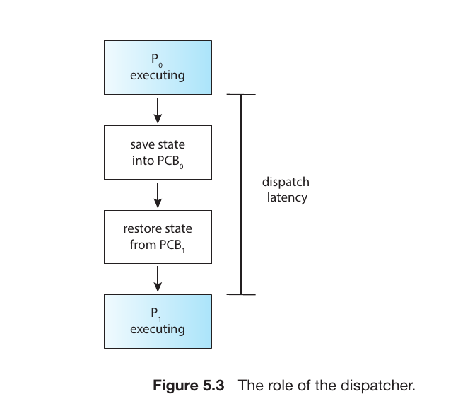
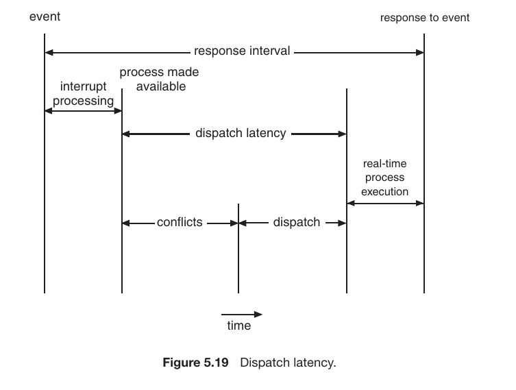
Dispatcher
While the Scheduler selects which process should run next, the Dispatcher is the module that actually gives control of the CPU to that selected process.
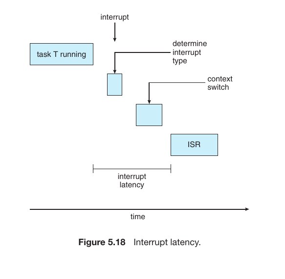
Fig.17
The Dispatcher’s Responsibilities:
Context Switching: Saving the state of the old process and loading the saved state for the new process.
Switching to User Mode: Transitioning the CPU from kernel mode back to user mode so the application can run.
Jumping: Moving to the specific location in the user program to resume execution from where it last stopped.
Dispatch Latency:
This is the time it takes for the dispatcher to stop one process and start another. To ensure a fast and responsive system, this latency must be as low as possible.
Scheduling Criteria
1. CPU Utilization
The goal is to keep the CPU as busy as possible. In an ideal world, utilization ranges from 0% to 100%. In a real-world system, it usually sits at 40% during light loads and can go up to 90% during heavy processing.
Goal:Maximize (keep the CPU working).
2. Throughput
Throughput is the number of processes that complete their execution per unit of time (e.g., per second or per minute). While throughput might be lower for long processes, it can be very high for shorter tasks.
Goal:Maximize (finish as many tasks as possible).
3. Turnaround Time
This is the total amount of time taken from the moment a process is submitted until it is completely finished. It includes:
Ready Queue Waiting Time + CPU Execution Time + I/O Time.
Goal:Minimize (finish the whole job quickly).
4. Waiting Time
Waiting time is the total period a process spends sitting idle in the Ready Queue waiting for its turn on the CPU. Scheduling algorithms have a direct and significant impact on this specific metric.
Goal:Minimize (reduce the time spent standing in line).
5. Response Time
In interactive systems, the total time to finish a task isn’t as important as how quickly the system starts responding. Response time is the duration between submitting a request and the first response produced.
Goal:Minimize (make the system feel “snappy” to the user).
5.3 Scheduling Algorithms
CPU scheduling is the process of deciding which process in the Ready Queue will be allocated to the CPU core. While modern processors have multiple cores, these algorithms are discussed here in the context of a single-core system for simplicity.
First-Come, First-Served (FCFS)
This is the simplest scheduling algorithm. The process that requests the CPU first is allocated the CPU first. It is managed using a FIFO (First-In-First-Out) queue.
Problem: The average waiting time is often quite long.
Convoy Effect: If a large CPU-bound process arrives first, all smaller I/O-bound processes get stuck behind it, leading to lower device utilization.
Type: This is a Non-preemptive algorithm (a process holds the CPU until it finishes or requests I/O).
Mathematical Example and Analysis
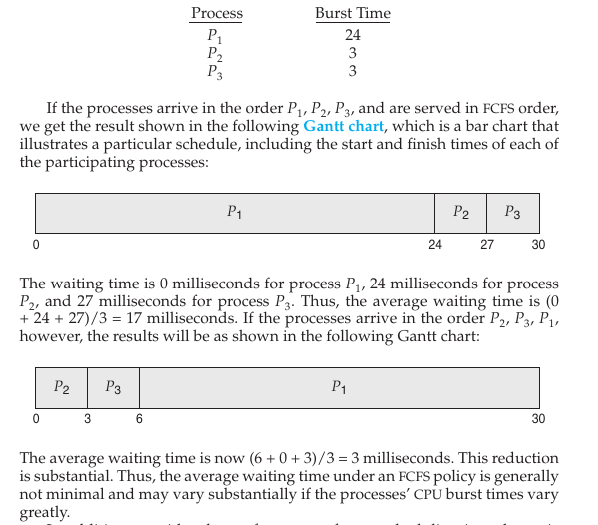
The example considers three processes ($P_1, P_2, P_3$) with the following Burst Times:
$P_1$: 24 ms
$P_2$: 3 ms
$P_3$: 3 ms
Scenario 1: Processes arrive in the order $P_1, P_2, P_3$
Scenario 2: Processes arrive in the order $P_2, P_3, P_1$
$P_2$ starts at 0 ms (0 ms wait).
$P_3$ starts at 3 ms (3 ms wait).
$P_1$ starts at 6 ms (6 ms wait).
Average Waiting Time: $(0 + 3 + 6) / 3 = 3$ ms.
Fig.18
The Convoy Effect
The text highlights a major disadvantage of FCFS known as the Convoy Effect.
This occurs when a large, CPU-bound process (like $P_1$) holds the CPU for a long time.
Smaller, I/O-bound processes get stuck behind the large process, waiting for their turn.
This results in low CPU and device utilization, as many processes are waiting for one big task to finish. It is similar to a line of fast cars being stuck behind a slow-moving heavy truck on a narrow road.
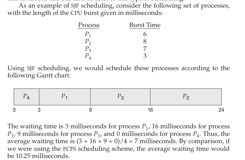
2. What is Shortest-Job-First (SJF)?
SJF is an algorithm that allocates the CPU to the process with the smallest Burst Time (the time required to complete its CPU cycle). If two processes have the same burst time, FCFS (First-Come, First-Served) is typically used as a tie-breaker.
Two Types of SJF
SJF operates in two distinct modes:
A. Non-preemptive SJF
In this mode, once a process is allocated the CPU, it holds it until it completes its current CPU burst. It cannot be interrupted by a new, shorter process.
Example: If we have processes with burst times of 6, 8, 7, and 3 ms, $P_4$ (3 ms) runs first because it is the shortest. Then $P_1$ (6 ms), followed by $P_3$ (7 ms), and finally $P_2$ (8 ms). In this case, the average waiting time is 7 ms.
Fig.19
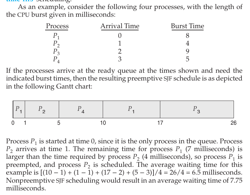
B. Preemptive SJF (Shortest-Remaining-Time-First - SRTF)
In this mode, if a new process arrives with a burst time shorter than the remaining time of the currently running process, the current process is interrupted (preempted), and the new process is given the CPU.
Example: $P_1$ starts at 0 ms with an 8 ms burst. After 1 ms, $P_2$ arrives with a 4 ms burst. Since $P_2$’s time (4 ms) is less than $P_1$’s remaining time (7 ms), $P_1$ is stopped, and $P_2$ takes over.
Fig.20
3. Predicting Future Burst Times (Exponential Averaging)
A significant challenge with SJF is that the length of the next CPU burst is difficult to know in advance. To solve this, the OS predicts the next burst using an exponential average of previous bursts:
$$\tau_{n+1} = \alpha t_n + (1 - \alpha)\tau_n$$
$\tau_{n+1}$: Predicted value for the next CPU burst.
$t_n$: Actual length of the most recent ($n^{th}$) CPU burst.
$\alpha$: A weight factor (usually $1/2$) used to balance the importance of recent history versus past history.
Feature
Description
Core Principle
The shortest task gets the CPU first.
Advantage
Guarantees the minimum average waiting time.
Disadvantage
Difficult to predict the next burst; larger processes may suffer from Starvation.
Preemptive Form
Also known as Shortest-Remaining-Time-First (SRTF).
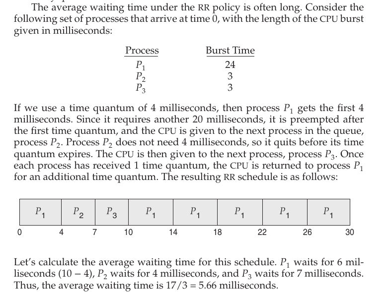
Round-Robin (RR) Scheduling
Designed specifically for time-sharing systems, this algorithm gives each process a small unit of CPU time called a Time Quantum (usually 10–100 milliseconds).
Process: After the time quantum expires, the process is preempted and added to the tail of the ready queue.
Performance: If the time quantum is too small, it causes excessive Context Switching, slowing down the system. If it is too large, it behaves exactly like FCFS.
A Practical Example (From the Image)
In the provided example, the Time Quantum is set to 4 ms. The processes are: $P_1$ (24 ms), $P_2$ (3 ms), and $P_3$ (3 ms).
$P_1$: It runs for the first 4 ms and is then preempted (remaining time: 20 ms).
$P_2$: Since it only requires 3 ms (which is less than the 4 ms quantum), it completes its task and finishes entirely.
$P_3$: Similarly, it runs for 3 ms and finishes.
$P_1$ Returns: Now, $P_1$ repeatedly receives 4 ms slices of CPU time until its remaining 20 ms are exhausted.
Fig.20
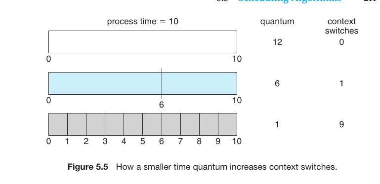
The Relationship Between Time Quantum and Context Switch
1. Large Time Quantum (Quantum = 12)
If the quantum is larger than the time required by the process, the process finishes in a single turn.
Context Switches: 0
Effect: It behaves exactly like FCFS (First-Come, First-Served).
2. Medium Time Quantum (Quantum = 6)
In this case, the 10-unit process needs two turns to finish (first 6 units, then the remaining 4).
Context Switches: 1
Effect: The process is interrupted once, adding a small amount of overhead.
3. Small Time Quantum (Quantum = 1)
If the quantum is very small, the process must return to the CPU 10 separate times to complete its 10-unit task.
Context Switches: 9
Effect: A massive amount of time is wasted on switching between processes, which significantly slows down the actual work.
Fig.21
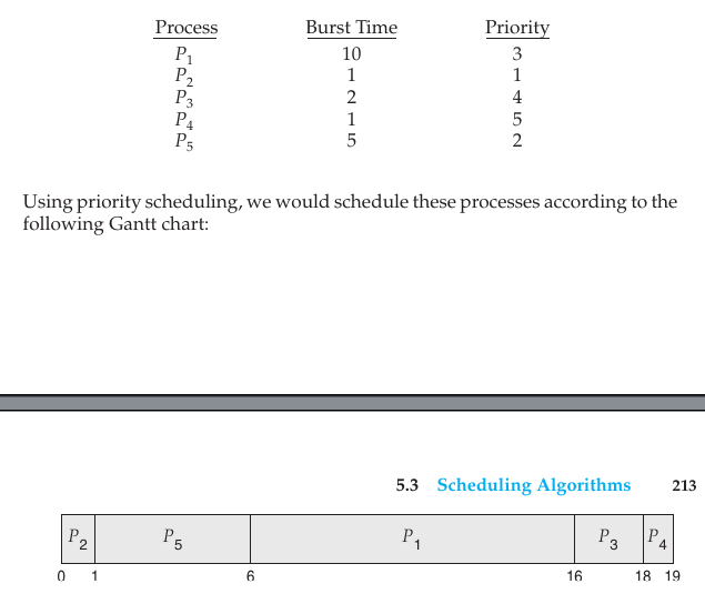
Priority Scheduling
A priority is associated with each process, and the CPU is allocated to the process with the highest priority (usually, a smaller integer represents a higher priority).
Starvation (Indefinite Blocking): Low-priority processes may stay in the ready queue indefinitely if higher-priority processes keep arriving.
Solution (Aging): Gradually increasing the priority of processes that wait in the system for a long time so they eventually get a chance to run.
Fig.21
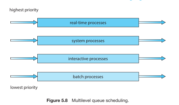
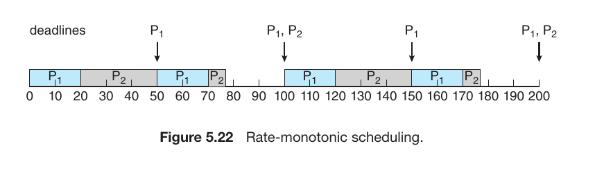
Multilevel Queue Scheduling
Instead of one single queue, processes are partitioned into separate queues based on their nature (e.g., Foreground/Interactive vs. Background/Batch).
Each queue can have its own scheduling algorithm (e.g., RR for foreground and FCFS for background).
Scheduling must also happen between queues, usually as fixed-priority preemptive scheduling.
Fig.22
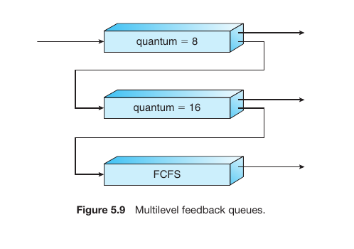
Multilevel Feedback Queue Scheduling
This is the most complex and flexible algorithm. Unlike a standard multilevel queue, processes can move between queues.
If a process uses too much CPU time, it is demoted to a lower-priority queue.
If a process waits too long in a lower-priority queue, it is promoted to a higher-priority queue (Aging).
This setup favors interactive tasks with short CPU bursts and leaves long, CPU-heavy tasks for the background.
Fig.23
Summary Comparison Table
Algorithm
Principle
Key Characteristic
FCFS
First come, first served
Simple but suffers from the Convoy Effect.
SJF
Shortest task goes first
Provides the lowest average waiting time.
RR
Fixed time sharing
Best for interactive/time-sharing systems.
Priority
Based on importance
Can lead to Starvation; fixed by Aging.
Multilevel
Separate queues()
Categorizes tasks by type (e.g., Batch vs. Interactive).
Feedback
Dynamic migration
Most flexible; prevents starvation and optimizes response.
Thread Scheduling
In modern operating systems, the scheduler primarily manages Threads rather than entire processes. Since there are two types of threads—User-level and Kernel-level—their scheduling is handled through two distinct scopes:
1. Contention Scope
This defines who the threads are competing against to gain CPU time.
Process-Contention Scope (PCS): This is applicable to User-level threads. Threads belonging to the same process compete with each other to be mapped onto an available LWP (Lightweight Process). This scheduling is managed by the Thread Library.
Analogy: Imagine 3 employees (threads) in a single office competing for only 1 available chair (LWP). The office manager (thread library) decides who sits down.
The Role of LWP (Lightweight Process)
The **LWP** acts as a bridge between User-level threads and Kernel-level threads.
* User threads cannot access the CPU directly.
* A User thread must first be bound to an **LWP**.
* The Operating System then schedules that LWP onto a physical CPU core.
System-Contention Scope (SCS): This applies to Kernel-level threads. Here, all kernel threads in the entire system compete against each other for the actual Physical CPU. The Operating System Kernel makes this decision.
Analogy: Now, all employees from every office in the city are competing for a limited number of seats across the whole country.
Multi-Processor Scheduling
When a system has multiple CPU cores, scheduling becomes significantly more complex than in a single-core system. The primary goal is to ensure all processors are utilized efficiently while maintaining a balanced workload.
Multi-Processor Architectures
The text also highlights how hardware design influences scheduling:
Multicore CPUs: Placing multiple computing cores on a single physical chip. This allows for faster communication and lower power consumption.
Multithreaded Cores (Hyper-threading): A single physical core acts as two logical processors. While one thread is waiting for memory (a memory stall), the core can switch to another thread instantly.
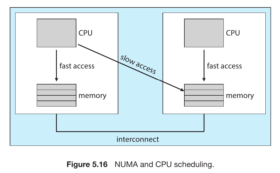
NUMA (Non-Uniform Memory Access): In systems with many CPUs, some parts of memory are “closer” to certain CPUs than others. The scheduler must be “NUMA-aware” to ensure a process runs on a CPU close to its data.
Asymmetric Multiprocessing (AMP)
In an Asymmetric system, there is a clear hierarchy. One processor is designated as the Master Server, while the others function as Slaves or subordinates.
Master’s Role: The master processor is the only one that handles system-wide tasks like scheduling, I/O processing, and other system activities.
Slave’s Role: The other processors only execute user code as directed by the master.
Symmetric Multiprocessing (SMP)
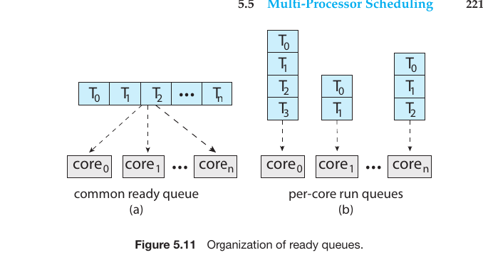
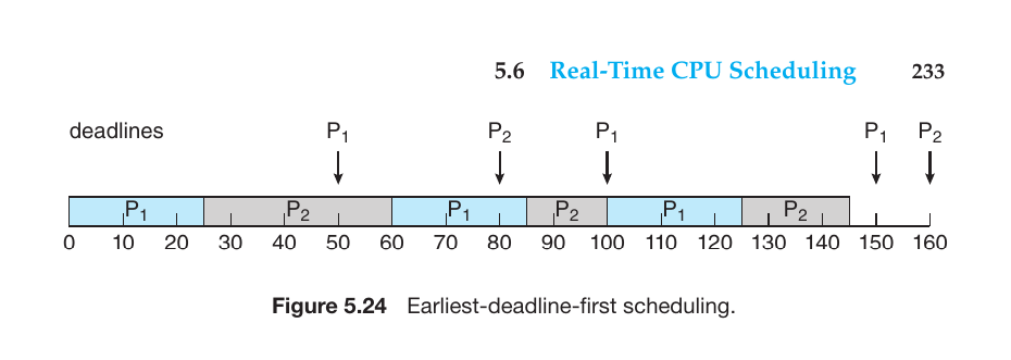
In modern operating systems (Windows, Linux, macOS), SMP is the standard. Here, each processor is self-scheduling. There are two primary ways to organize the ready threads:
A. Common Ready Queue
All threads wait in a single, shared queue. Any available processor picks a task from this global line.
Pros: Naturally balances the workload.
Cons: Leads to performance bottlenecks due to Race Conditions. To prevent two processors from picking the same task, the queue must be “locked,” which slows down the system.
B. Per-Core Run Queues
Each core maintains its own private queue of tasks.
Pros: This is the most popular method in modern OS architecture. It reduces contention between cores and improves Cache Affinity (keeping a task on the same core so its data stays in the local cache).
Cons: Can lead to Load Imbalance, where one core is overwhelmed while another is idle. This requires specific Load Balancing algorithms (Push/Pull migration).
Fig.24
Symmetric vs. Asymmetric Comparison
Feature
Asymmetric (AMP)
Symmetric (SMP)
Decision Maker
Only the Master Processor.
Each Processor decides for itself.
Complexity
Simple to design.
Complex to implement.
Bottleneck
High risk (Master gets overwhelmed).
Low risk (Workload is shared).
Modern Usage
Rarely used in main OS; found in specialized hardware.
Used in Windows, Linux, macOS, Android.
Memory Stall and Chip Multithreading (CMT)
In modern computing, processors are much faster than the memory (RAM) they talk to. This creates a significant performance gap.
1. What is a Memory Stall?
A Memory Stall occurs when a processor core has to stop executing instructions because it is waiting for data to arrive from memory.
The Problem: As shown in your reference images, a processor can spend up to 50% of its time doing nothing but waiting (stalling). This is a massive waste of high-speed hardware resources.
2. Chip Multithreading (CMT)
To solve this, hardware designers introduced Chip Multithreading (CMT). Instead of having just one sequence of execution, a single physical core is designed to hold multiple Hardware Threads (Logical Processors).
How it Works:
If Thread 0 encounters a memory stall, the core doesn’t sit idle.
It immediately switches to Thread 1 and starts executing its instructions.
By the time Thread 1 finishes or stalls, the data for Thread 0 has likely arrived, and the core can switch back.
Fig.25
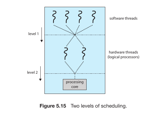
Two level scheduling in os
For Hyper-threading ther are two level scheduling in os
Level 1: Operating System (Software) Level
At this level, the OS scheduler decides which Software Thread should be assigned to which Logical Processor.
The OS View: The Operating System (Windows, Linux, etc.) doesn’t see “Physical Cores”; it only sees Logical Processors (Hardware Threads).
Task Management: If you have 4 cores with Hyper-threading, the OS sees 8 CPUs. It tries to spread the workload across all 8 to keep the system responsive.
Level 2: Hardware (Core) Level
At this level, the physical CPU hardware decides how to execute the instructions from the two logical processors assigned to a single core.
Resource Sharing: Two logical processors on the same core share the same execution units (ALUs, FPUs) and caches (L1, L2).
Latency Hiding: As you mentioned earlier regarding Memory Stalls, the hardware level is responsible for switching between logical processors in nanoseconds. If Logical Processor 0 is waiting for RAM, the hardware instantly lets Logical Processor 1 use the execution units.
Fig.26
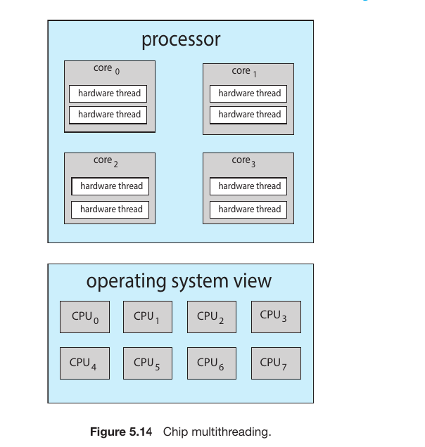
3. Intel Hyper-threading
This is the most well-known commercial example of CMT.
Logic: To the Operating System, a 4-core processor with Hyper-threading looks like an 8-core processor.
Figure 5.14: As you mentioned, if a system has 4 physical cores and each core has 2 hardware threads, the OS sees 8 logical CPUs. This allows the OS scheduler to push more tasks into the “pipeline” to keep the hardware busy.
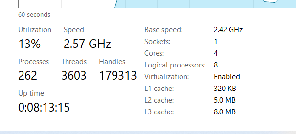
My task manager figure
Fig.27
Sockets: 1 – This confirms you have one physical CPU chip installed on your motherboard.
Cores: 4 – Inside that single chip, there are 4 independent physical processing units.
Logical Processors: 8 – This is the most interesting part. Because of Hyper-threading, each physical core acts as two logical units. The Operating System “believes” it has 8 separate CPUs available to handle work.
L1, L2, and L3 Cache – These are the ultra-fast memory layers built into the CPU. The processor checks these first to avoid the Memory Stalls we discussed earlier. If the data isn’t in the cache, it has to wait for the much slower RAM.
Load Balancing vs. Processor Affinity
In a Multi-processor system (SMP), the final challenge for the OS is deciding whether to move a task to keep CPUs busy or keep a task where it is to maintain speed.
1. Load Balancing
Load balancing ensures that no single processor is overloaded while others sit idle. It uses two main strategies:
Push Migration: A specific system task periodically monitors the workload. If it finds a “bottleneck” on one processor, it forcibly pushes threads to a less busy processor.
Pull Migration: When a processor finishes all its tasks and becomes idle, it actively pulls a waiting task from the queue of a busy processor.
2. Processor Affinity
Affinity is the tendency of a thread to stay on the same processor.
Warm Cache: While a thread runs on CPU-0, that CPU’s cache fills up with the thread’s data.
The Problem: If Load Balancing moves that thread to CPU-1, the “warm” cache is lost. CPU-1 must spend time fetching data from slow RAM to rebuild its own cache.
The Goal: Affinity tries to keep a thread on the same processor to maximize cache efficiency.
3. NUMA and Scheduling
In NUMA (Non-Uniform Memory Access) systems, the physical distance between a CPU and a memory module matters.
Local Memory: A CPU can access its own assigned memory very quickly.
Remote Memory: Accessing memory assigned to another CPU is much slower.
The Strategy: A “NUMA-aware” scheduler ensures a thread is scheduled on the CPU that is physically closest to the memory where its data is stored.
Fig.27
Heterogeneous Multiprocessing (HMP)
we have discussed Homogeneous systems where every CPU core is identical. However, in HMP, not all cores are created equal. This technology is the backbone of modern smartphones and power-efficient laptops.
1. The big.LITTLE Architecture
Developed primarily by ARM, this architecture uses two distinct types of cores within a single physical processor:
big cores: High-performance, high-clock-speed cores designed for maximum processing power. They consume a significant amount of battery.
LITTLE cores: Energy-efficient, lower-clock-speed cores. They handle background tasks while consuming very little power.
2. How the HMP Scheduler Works
In an HMP system, the OS scheduler must be much “smarter” because it doesn’t just decide when to run a task, but where to run it based on its priority and power needs:
Heavy Tasks: If you are gaming or rendering high-definition video, the scheduler assigns the threads to the big cores for maximum performance.
Light Tasks: For background syncs, checking emails, or playing music, the scheduler moves the threads to the LITTLE cores to conserve energy.
Battery Saver Mode: When your device is low on power, the OS can disable the “big” cores entirely, forcing all tasks onto the power-sipping “LITTLE” cores to keep the device alive.
3. Benefits of HMP
Feature
Description
Power Efficiency
Significant battery savings by not using high-power cores for trivial tasks.
Thermal Management
Reduces heat generation, preventing the device from getting uncomfortably hot.
Burst Performance
When necessary, the system can engage all cores (big and LITTLE) simultaneously for peak processing.
Real-Time CPU Scheduling
In real-time systems, the correctness of a computation depends not only on the logical result but also on the time at which the result is delivered. Meeting a Deadline is the primary goal.
1. Types of Real-Time Systems
Soft Real-Time Systems: These provide no guarantee as to when a critical real-time process will be scheduled. They only guarantee that the process will be given preference over non-critical processes.
Example: Multimedia streaming or online gaming.
Hard Real-Time Systems: These have strict requirements. A task must be serviced by its deadline; failure to meet the deadline is considered a total system failure.
Example: Nuclear power plant controllers, medical imaging systems, or automotive airbags.
2. Understanding Latency
In real-time scheduling, minimizing Event Latency is crucial. As you noted, there are two main components:
Interrupt Latency: The period from the arrival of an interrupt at the CPU to the start of the routine that services the interrupt.
Fig.28
Dispatch Latency: The time it takes for the dispatcher to stop one process and start another. To be effective, real-time operating systems keep this latency extremely short by making system calls preemptible.
Fig.27
3. Real-Time Scheduling Algorithms
Standard scheduling isn’t enough; we need algorithms that understand periods ($P$), burst times ($t$), and deadlines ($d$).
A. Rate-Monotonic (RM) Scheduling
This uses Static Priority.
The Rule: Priorities are assigned based on the inverse of the period. The shorter the period, the higher the priority.
Logic: Tasks that occur more frequently are deemed more urgent.
Fig.27
Rate-Monotonic Scheduling, the priority of a task is determined based on its Period (the time interval).
The shorter the period, the higher the priority.
In this case, the period of $P_1$ is 50, and the period of $P_2$ is 100.
Since 50 is less than 100, $P_1$ is assigned a higher priority.
Step-by-Step Breakdown
1. Time 0 to 20 ($P_1$ executes):
At the very beginning (time 0), both $P_1$ and $P_2$ are ready. However, because $P_1$ has a higher priority, it starts first and completes its task in 20 units.
2. Time 20 to 50 ($P_2$ executes):
Since $P_1$ has finished its work, the CPU becomes idle. $P_2$ now begins its execution. $P_2$ requires a total of 35 units. It manages to complete 30 units of work from time 20 to 50, leaving 5 units of work remaining.
3. Time 50 (Preemption):
At time 50, process $P_1$ arrives again for its next cycle. According to the rules, $P_1$ has a higher priority, so it interrupts (preempts) the currently running $P_2$ and takes control of the CPU. This is known as Preemption.
4. Time 50 to 70 ($P_1$ executes):
$P_1$ completes its second round of work, which takes 20 units of time.
5. Time 70 to 75 ($P_2$ finishes):
Once $P_1$ finishes, $P_2$ gets the chance to complete its remaining 5 units of work. $P_2$ finally finishes at 75 minutes, which is well before its deadline of 100 minutes.
6. Time 75 to 100 (Idle Time):
During this interval, there are no active tasks, so the CPU remains idle. At the 100-minute mark, both processes will restart their cycles again.
B. Earliest-Deadline-First (EDF) Scheduling
This uses Dynamic Priority.
The Rule: Priorities are assigned according to the deadline. The earlier the deadline, the higher the priority.
Logic: When a new task becomes ready, the scheduler adjusts priorities so that the task closest to its “expiration” runs first.
Fig.27
Detailed Breakdown
This example uses the same processes that failed under Rate-Monotonic scheduling ($P_1$: Period 50, Burst 25; and $P_2$: Period 80, Burst 35).
1. Time 0 to 25 ($P_1$ starts):
At the beginning, $P_1$ has a deadline of 50, and $P_2$ has a deadline of 80. Since 50 is earlier than 80, $P_1$ executes first and finishes at time 25.
2. Time 25 to 50 ($P_2$ starts):
The CPU is now free, so $P_2$ begins its task. At the 50-minute mark, $P_1$ arrives again for its next cycle.
3. The Major Change (At Time 50):
In Rate-Monotonic: $P_1$ would have preempted $P_2$ because $P_1$ has a shorter period.
In EDF: At time 50, $P_1$’s next deadline is 100 ($50+50$), while $P_2$’s current deadline is 80. Since 80 is earlier than 100, EDF does not interrupt $P_2$. $P_2$ continues until time 60 and finishes its work.
4. Time 60 to 85 ($P_1$’s second burst):
Once $P_2$ finishes, $P_1$ starts its 25-unit burst and completes at time 85 (well before its deadline of 100).
5. Time 85 to 145:
At time 80, $P_2$ arrived again with a new deadline of 160 ($80+80$). Meanwhile, $P_1$’s next deadline is 150. Since 150 is earlier than 160, $P_1$ starts again at time 100. The scheduler continues to prioritize whoever has the nearest upcoming deadline.
Proportional Share Scheduling
Proportional Share Scheduling is a scheduling method where the total available CPU time is divided into a fixed number of “Shares” and distributed among various processes.
Share Distribution
Imagine the total number of shares is $T = 100$. Now, consider three processes:
Process A: Allocated 50 shares.
Process B: Allocated 15 shares.
Process C: Allocated 20 shares.
This means Process A will receive 50% of the total CPU time, Process B will receive 15%, and Process C will receive 20%.
Three critical methods for evaluating CPU scheduling algorithms are discussed:
Queueing Models
Simulations
Implementation
1. Queueing Models
Since real-world processes vary unpredictably, we use mathematical probability to estimate performance. This is known as Queueing-Network Analysis.
Little’s Formula
The most fundamental equation in this model is Little’s Formula:
$$n = \lambda \times W$$
$n$: Average queue length (number of processes in the queue).
$\lambda$ (Lambda): Average arrival rate for new processes.
$W$: Average waiting time in the queue.
Example: If 7 new processes arrive every second ($\lambda = 7$) and the queue typically holds 14 processes ($n = 14$), then each process waits an average of 2 seconds ($W = 14 / 7 = 2$).
2. Simulations
When mathematical formulas are too simple to capture complex system behavior, we use Simulations.
How it works: A software model of the computer system is created. A variable representing a “clock” is incremented, and the simulator tracks the state of the CPU, I/O devices, and the scheduler.
Trace Files: To make simulations accurate, researchers record the behavior of real processes on an actual system (e.g., exactly when they use the CPU or perform I/O). This recorded data is called a Trace File. By running different algorithms against the same trace file, we can see exactly which one performs better under real-world conditions.
3. Implementation
This is the most accurate but also the most difficult and expensive method. It involves writing the actual code for the algorithm and putting it into a real Operating System.
The Challenge: It is risky; a bug in the scheduler can crash the entire system. It is also time-consuming to compile and test a full OS kernel.
User Behavior: Interestingly, when you change an algorithm, users change their behavior. For example, if a scheduler favors short jobs, programmers might break their large programs into many small pieces to “cheat” the system and get faster service.
Tuning: Some systems provide tools (like the dispadmin command in Solaris) that allow administrators to “tune” or adjust scheduling parameters without rewriting the code.
Comparison of Evaluation Methods
Method
Accuracy
Complexity / Cost
Deterministic Modeling
Low (Only for specific data)
Very Simple & Fast
Queueing Models
Moderate (Probabilistic)
Mathematically Complex
Simulations
High (Especially with Trace Files)
High Time & Storage Costs
Implementation
Highest (Real-world results)
Extremely Complex & Risky
The Bounded-Buffer Problem, which is a classic multi-process synchronization challenge.
This problem involves two parties—the Producer and the Consumer—who share a common, fixed-size buffer (memory space).
Producer: Generates data and places it into the buffer.
Consumer: Takes data out of the buffer to use it.
The Problem: The Producer must not add data if the buffer is full, and the Consumer must not remove data if the buffer is empty. To prevent conflicts and data corruption (Race Conditions), synchronization via Semaphores is required.
2. Data Structures Used
To solve this problem, three specific semaphores are utilized:
int n: The total capacity of the buffer.
semaphore mutex = 1: Provides Mutual Exclusion. It acts as a “lock,” ensuring that only one process (either Producer or Consumer) can access the buffer at any given time.
semaphore empty = n: Keeps track of the number of empty slots. It starts at $n$ (because the buffer is initially empty).
semaphore full = 0: Keeps track of the number of occupied slots. It starts at $0$.
3. The Producer Process
The Producer follows these steps to safely add an item:
Produce an item.
wait(empty): Checks if there is an empty slot. If empty > 0, it decrements the count and proceeds. If not, it waits.
wait(mutex): Locks the buffer to prevent the Consumer from entering.
Add the item to the buffer.
signal(mutex): Unlocks the buffer.
signal(full): Increments the count of full slots to notify the Consumer that new data is available.
Readers-Writers Logic
The unique feature here is concurrency for readers. Unlike the Bounded-Buffer where only one person can touch the data at a time, here:
The First Reader locks the door (rw_mutex) to keep writers out.
Other Readers can enter freely without needing to lock anything.
The Last Reader to leave is the only one who unlocks the door so a writer can finally enter.
the Dining-Philosophers Problem,
a classic synchronization challenge that represents the difficulties of sharing multiple resources among several processes.
1. The Scenario
Five Philosophers: Sitting around a circular table, they spend their lives alternating between two states: Thinking and Eating.
The Setting: A bowl of rice is in the center, and there are five single chopsticks placed on the table, one between each pair of philosophers.
The Rule of Eating: When a philosopher gets hungry, they try to pick up their left and right chopsticks. They can only eat if they successfully hold both at the same time.
Post-Eating: Once they finish eating, they place both chopsticks back on the table and return to thinking.
2. The Core Challenge: Deadlock
While the rules seem simple, they lead to a major synchronization failure known as a Deadlock.
Deadlock Situation: Imagine all five philosophers become hungry at the exact same time. Each one reaches out and picks up the chopstick to their left.
The Result: Now, every philosopher is holding one chopstick and waiting for the one on their right. Since all chopsticks are already held, no one can pick up a second one.
The Consequence: Everyone waits forever for a resource that will never be released. This “circular wait” is the definition of a Deadlock, where the system grinds to a complete halt because every process is stuck waiting for another.
The semaphore-based solution for the Dining-Philosophers Problem
1. The Semaphore Solution
In this approach, each chopstick is represented as an individual semaphore.
Shared Data:semaphore chopstick[5]; (All initialized to 1).
Execution: A philosopher executes a wait() operation to pick up a chopstick and a signal() operation to release it after eating.
2. The Major Flaw: Deadlock
While this method prevents two neighbors from eating simultaneously, it is highly susceptible to a Deadlock.
The Scenario: If all five philosophers become hungry at the same time and pick up their left chopstick, all semaphore values become 0.
The Result: When they attempt to pick up their right chopstick, every philosopher is “delayed forever” because no chopsticks are available. The system reaches a total standstill.
3. Remedies for Deadlock
To ensure the system remains functional, one of these three strategies must be implemented:
1. Limiting the Number of Seats
The Concept: If 5 philosophers sit at a table with 5 chopsticks, they can each grab one and cause a deadlock. By limiting the seats to 4, we guarantee that at least one person can always access two chopsticks.
Example:
4 philosophers ($P_1, P_2, P_3, P_4$) sit down, but there are still 5 chopsticks on the table.
Even if everyone picks up one chopstick, 4 are taken and 1 is still on the table.
This 5th chopstick allows one of the philosophers to complete their pair, eat, and then release both chopsticks for others.
2. Pick Up Only if Both are Available
The Concept: A philosopher will not pick up a single chopstick unless they are certain that both the left and right ones are free. This check happens inside a Critical Section to ensure no one else grabs a chopstick while they are checking.
Example:
Philosopher $P_1$ is hungry. They see the left chopstick is free, but the right one is being used by a neighbor.
Instead of picking up the left one and waiting (which leads to deadlock), $P_1$ waits without picking up anything.
By keeping their hands off the table until both tools are ready, they prevent the “hold and wait” situation.
3. Asymmetric Solution
The Concept: Deadlocks often happen because everyone moves in the same direction (symmetry). By making Odd and Even numbered philosophers follow different rules, we break that symmetry.
Example:
Odd Philosophers ($P_1, P_3, P_5$): They reach for the Left chopstick first, then the Right.
Even Philosophers ($P_2, P_4$): They reach for the Right chopstick first, then the Left.
The Result: Imagine $P_1$ and $P_2$ sitting next to each other. They share one chopstick between them. Because they reach in opposite directions, one will grab it first while the other is forced to wait before they can even pick up their first chopstick. This prevents the “Circular Wait.”
The Monitor-based solution is to be Deadlock-free.
It achieves this by enforcing a strict rule: A philosopher is allowed to pick up their chopsticks only if both the left and right chopsticks are currently available.
2. Shared Data Structures
The Monitor manages the state of the philosophers using two key structures:
State Array:enum {THINKING, HUNGRY, EATING} state[5];
This tracks the status of each philosopher.
Philosopher $i$ can only set their state to EATING if:
The neighbor on the left is not eating: state[(i+4) % 5] != EATING
The neighbor on the right is not eating: state[(i+1) % 5] != EATING
Condition Variables:condition self[5];
If a philosopher is HUNGRY but their neighbors are eating, they call self[i].wait(). This suspends them until a neighbor finishes eating and signals them to wake up.
3. The Execution Sequence
To interact with the shared chopsticks, a philosopher must call the Monitor’s procedures in this specific order:
Pickup(i): Sets the state to HUNGRY, checks if neighbors are eating, and either starts eating or waits.
Eat: The philosopher performs their actual task (eating).
Putdown(i): Sets the state back to THINKING and, crucially, checks if the left or right neighbors are hungry and can now eat. If so, it signals them.
4. Strengths and Weaknesses
Success: Deadlock Prevention
Because no philosopher “holds” one chopstick while “waiting” for another (they only grab both or none), the Circular Wait condition is broken. This makes the solution completely deadlock-free.
Limitation: Starvation
While the system will never freeze (no deadlock), it does not guarantee Fairness.
The Scenario: If Philosopher $i$ is hungry, but their neighbors (left and right) take turns eating in such a way that there is never a moment when both are thinking at the same time, Philosopher $i$ will starve.
Syncronization in kernel
1. Kernel-Level Synchronization
The Windows kernel must manage shared data across multiple CPU cores efficiently. It uses two primary techniques:
Interrupt Masking: On single-processor systems, the kernel temporarily “masks” (turns off) interrupts. This ensures that a critical task isn’t interrupted halfway through.
Spinlocks: On multi-processor systems, the kernel uses spinlocks. To maintain speed, these are only used for very short sections of code. While a thread holds a spinlock, it is never preempted (interrupted by the scheduler), ensuring it finishes its task as fast as possible.
2. Dispatcher Objects (Synchronization for Apps)
For general thread synchronization, Windows uses Dispatcher Objects. These act as Mutexes, Semaphores, Events, and Timers. They exist in one of two states:
Signaled State: The object is available. A thread can acquire it without waiting.
Nonsignaled State: The object is busy. Any thread trying to acquire it will be moved to a Waiting Queue and put to sleep to save CPU cycles.
3. Events and Timers
Events: These act like condition variables. When a specific condition is met (like a file finishing its download), the event notifies waiting threads to wake up.
Timers: Used to notify threads after a specific amount of time has passed.
4. Critical-Section Objects (The Efficiency King)
This is one of the smartest features in Windows. It is a User-mode mutex that tries to avoid expensive calls to the Kernel.
The “Spin-then-Sleep” Strategy: In a multi-processor system, if a resource is busy, the thread first spins (loops) for a short time, hoping the resource becomes free. Spinning is “cheap” because it doesn’t involve the Kernel.
Falling Back: If the resource is still busy after spinning, only then does it allocate a Kernel Mutex and put the thread to sleep. This is highly efficient because the heavy Kernel overhead is only used when there is high competition (contention) for a resource.
Definition of Deadlock
In a multiprogramming environment, several threads may compete for a finite number of resources (such as printers, memory, or locks). A deadlock occurs when a process or thread enters a waiting state because the requested resources are held by other waiting threads, which in turn are waiting for resources held by the first process.
In simple terms: A situation where every process in a set is waiting for an event that can only be caused by another process in that same set. As a result, none of the processes can ever proceed.
2. Real-World Example (The Kansas Law Illustration)
The text highlights a famous (and likely anecdotal) law passed by the Kansas legislature in the early 20th century to illustrate this concept:
“When two trains approach each other at a crossing, both shall come to a full stop and neither shall start up again until the other has gone.”
If both trains follow this law strictly, they will both wait forever for the other to move first. Neither can proceed because the “event” they are waiting for (the other train leaving) can never happen. This perfectly mirrors a deadlock in an operating system.
The System Model
is a structured way of describing how threads interact with resources. It assumes that a thread cannot use more than the total number of available resources and must follow the Request $\rightarrow$ Use $\rightarrow$ Release protocol.
The Resource Utilization Cycle
A thread may utilize a resource only in the following sequence. If this sequence is blocked indefinitely for a set of threads, a deadlock is formed.
Request: The thread requests the resource. If the request cannot be granted immediately (e.g., all instances are being held by other threads), the requesting thread must wait until it can acquire the resource.
Use: Once the thread has successfully acquired the resource, it operates on it (e.g., if the resource is a printer, the thread starts printing).
Release: After the thread has finished using the resource, it must release it so that the instance becomes available for other threads in the system.
Understanding Livelock
Livelock is a specific type of liveness failure where two or more threads are unable to proceed because they are continuously reacting to each other’s actions. Unlike a deadlock, where threads are blocked and waiting, threads in a livelock are active but making no progress.
Human Analogy: Imagine two people meeting in a narrow hallway. If both move to their right to let the other pass, they still block each other. If they then both move to their left at the same time, they continue to obstruct progress. They are moving, but neither can get past the other.
Technical Example: This can occur when using pthread_mutex_trylock(). If two threads acquire one mutex each and then attempt to acquire a second one using trylock(), the function fails if the second mutex is already held. If the threads are programmed to release their first mutex and retry the entire sequence every time a trylock() fails, they may repeat this cycle indefinitely.
Deadlock in Multithreaded Applications
A Deadlock occurs when a set of threads is stuck because every thread in the set is waiting for a resource that is currently held by another thread in that same set.
Real-World Example (Dining Philosophers): As shown in the classic Dining Philosophers problem, if every philosopher becomes hungry at the same time and picks up the chopstick to their left, there will be no chopsticks left on the table. Each philosopher will then wait indefinitely for the chopstick to their right to be released by their neighbor, creating a complete halt in progress.
Four Necessary Conditions for Deadlock
A deadlock situation can arise if and only if the following four conditions hold simultaneously in a system. If any one of these conditions is prevented, a deadlock cannot occur.
Mutual Exclusion: At least one resource must be held in a non-sharable mode. This means only one thread at a time can use the resource (e.g., a printer).
Hold and Wait: A thread must be holding at least one resource and waiting to acquire additional resources that are currently being held by other threads.
No Preemption: Resources cannot be taken away by force from a thread. A resource can only be released voluntarily by the thread holding it after that thread has completed its task.
Circular Wait: A set of waiting threads ${T_0, T_1, \dots, T_n}$ must exist such that $T_0$ is waiting for a resource held by $T_1$, $T_1$ is waiting for a resource held by $T_2$, and $T_n$ is waiting for a resource held by $T_0$.
2. Resource-Allocation Graph
Deadlocks can be described more precisely using a directed graph called a Resource-Allocation Graph. This graph consists of a set of vertices $V$ and a set of edges $E$.
Nodes (Vertices):
Threads ($T$): Represented as circles ${T_1, T_2, \dots, T_n}$.
Resource Types ($R$): Represented as rectangles ${R_1, R_2, \dots, R_m}$. Dots inside the rectangle represent individual instances of that resource type.
Edges:
Request Edge ($T_i \rightarrow R_j$): A directed edge from a thread to a resource type indicates the thread has requested an instance and is currently waiting.
Assignment Edge ($R_j \rightarrow T_i$): A directed edge from a resource instance to a thread indicates the resource has been allocated to that thread.
Fig.28
Fig.29

3. Identifying Deadlock from the Graph
The existence of a cycle in the graph is a key indicator of a deadlock:
If the graph contains no cycles: There is no deadlock in the system.
If the graph contains a cycle:
If there is only one instance per resource type, then a deadlock has occurred.
If there are multiple instances per resource type, a cycle indicates the possibility of a deadlock, but it is not guaranteed (some threads in the cycle might release resources eventually).
1. Three Main Approaches to Handling Deadlocks
According to the text, the deadlock problem can be addressed in three ways:
Ignore the Problem: Assume that a deadlock will never occur. Most operating systems (such as Windows and Linux) use this method because deadlocks happen infrequently, and the cost of preventing them is very high.
Prevention and Avoidance: Use specific protocols to ensure that the system never enters a deadlocked state.
Detection and Recovery: Allow deadlocks to occur, but implement mechanisms to detect them and recover from them once they happen.
2. Deadlock Prevention vs. Avoidance
There are two distinct methods used to ensure that a system never reaches a deadlock:
Method
How it Works
Deadlock Prevention
Ensures that at least one of the four necessary conditions for deadlock is made impossible.
Deadlock Avoidance
The OS has advance information about which resources a thread might request in the future. The OS calculates whether granting a request will keep the system in a “Safe State.”
3. Detection and Recovery
If no prevention or avoidance mechanisms are in place, a deadlock may occur. In such cases, the system must perform two tasks:
Run an algorithm to examine the state of the system and determine if a deadlock has occurred.
If a deadlock is detected, run a recovery algorithm to break the deadlock and return the system to normal operation.
Why do OSs “Ignore” Deadlocks?
Although ignoring the problem doesn’t seem like an ideal solution, it is popular for several reasons:
Cost and Performance: Constantly running prevention or avoidance algorithms puts a heavy load on the system and decreases overall performance.
Rare Occurrence: In many systems, deadlocks may only happen once a month. Running expensive algorithms 24/7 for such a rare event is often considered wasteful.
Manual Restart: If a system becomes unresponsive due to a deadlock, the user can simply perform a manual restart to temporarily resolve the issue.
the four necessary conditions for a Deadlock to occur and provide protocols for Deadlock Prevention
by invalidating at least one of these conditions.
Mutual Exclusion
For a deadlock to occur, at least one resource must be non-sharable (meaning only one process can use it at a time).
Prevention Strategy: If we could make all resources sharable (like read-only files), deadlocks would never happen.
The Reality: Unfortunately, some resources are inherently non-sharable by nature (e.g., a Mutex lock or a printer). Therefore, it is almost impossible to prevent deadlocks solely by attacking this condition.
Hold and Wait
A deadlock occurs when a process holds at least one resource and waits for another that is currently held by another process.
Protocol 1: A process must request and be allocated all its required resources before it begins execution.
Protocol 2: A process can request a new resource only when it has none currently allocated to it (it must release current resources before requesting others).
Disadvantages: These methods lead to low resource utilization (resources are held even when not in use) and may cause starvation, where a process waits indefinitely for all its required resources to be available simultaneously.
No Preemption
This condition states that resources cannot be forcibly taken from a process; they must be released voluntarily.
Prevention Strategy: If a process holding some resources requests another resource that cannot be immediately allocated, all resources currently held by that process are preempted (forcibly released).
Recovery: The process will only restart when it can regain its old resources along with the new ones it is requesting. This approach is commonly used for resources whose state can be easily saved and restored, such as CPU registers or memory.
Circular Wait
This condition involves a set of processes waiting for each other in a circular chain.
Prevention Strategy: Impose a total ordering of all resource types. Each resource is assigned a unique integer (e.g., $F(\text{disk_drive}) = 1$, $F(\text{printer}) = 5$).
The Rule: A process can only request resources in an increasing order of enumeration. If a process holds resource $R_i$, it can only request $R_j$ if $F(R_j) > F(R_i)$.
Result: By following this strict hierarchy, it becomes mathematically impossible to form a cycle in the resource-allocation graph.
Deadlock Avoidance
is a strategy that ensures a system never enters a deadlocked state by using advance information about resource requests. Unlike Deadlock Prevention, which imposes strict rules on how resources are handled, Avoidance focuses on dynamic decision-making.
Deadlock Avoidance
A Priori Information: The system must know in advance the maximum number of resources of each type that a process may need.
Dynamic Check: Every time a process requests a resource, the OS performs a calculation. It determines if granting the request will leave the system in a Safe State. If granting the request could potentially lead to a deadlock in the future, the process is forced to wait, even if the resource is currently available.
Resource-Allocation State: The system constantly monitors three specific factors to make these decisions:
The number of available resources of each type.
The number of resources currently allocated to each process.
The maximum future demands of each process.
A Safe State? (that include Deadlock avoidance)
A system is in a Safe State if the operating system can find an order (sequence) in which every thread can be allocated its maximum required resources without causing a deadlock. this specific order is called a Safe Sequence.
Safe State: A state where there is no risk of deadlock.
Unsafe State: A state where there is a possibility of deadlock, though it is not guaranteed. (Not all unsafe states lead to deadlocks, but all deadlocks originate from an unsafe state).
Deadlock: A specific subset of an unsafe state where the system is completely stuck.
Explanation through an Example
Consider a system with a total of 12 resources and three threads ($T_0, T_1, T_2$).
Thread
Max Need
Currently Allocated
Remaining Need
$T_0$
10
5
5
$T_1$
4
2
2
$T_2$
9
2
7
Total
9 (Allocated)
3 (Free)
Why is this a Safe State?
The system has 3 free resources. If we follow this sequence, everyone can finish:
Help $T_1$ first: $T_1$ needs 2 more. We have 3, so we give them 2. $T_1$ finishes and releases all 4 of its resources. Now we have 5 free resources ($3-2+4=5$).
Help $T_0$ next: $T_0$ needs 5 more. We have exactly 5 free. $T_0$ finishes and releases all 10 of its resources. Now we have 10 free resources.
Help $T_2$ last: $T_2$ needs 7 more. We have 10, so $T_2$ can easily finish.
Since a Safe Sequence $<T_1, T_0, T_2>$ exists, the system is in a Safe State.
3. When does it become an Unsafe State?
The image explains that if the system mistakenly gave just one more resource to $T_2$ (even though it is currently free), the system would be left with only 2 free resources. While $T_1$ could still finish, the remaining resources would not be enough to satisfy the needs of either $T_0$ or $T_2$. The system would then enter an Unsafe State, creating a high risk of deadlock.
Resource-Allocation Graph (RAG) Algorithm
for deadlock avoidance is used specifically in systems where each resource type has only a single instance(Like one printer or one thread).
The Claim Edge
In this algorithm, a new type of edge is introduced called a Claim Edge ($T_i \rightarrow R_j$).
Representation: It is drawn as a dashed line.
Meaning: It indicates that thread $T_i$ may request resource $R_j$ at some point in the future.
Requirement: All claim edges for a thread must appear in the resource-allocation graph before the thread starts executing.
2. How the Algorithm Works
The algorithm manages the transition of edges to decide whether it is safe to grant a resource:
Request: When thread $T_i$ actually requests resource $R_j$, the dashed Claim Edge converts into a solid Request Edge.
Allocation Check: Before converting the Request Edge into an Assignment Edge (allocating the resource), the system checks for cycles.
Cycle Detection: The request is only granted if converting the edge does not result in a cycle in the graph.
Fig.29
Banker’s Algorithm Overview
The Banker’s Algorithm is used for deadlock avoidance in systems with multiple instances of resource types.
Each process must declare its Maximum resource needs upfront.
The OS only grants a request if the system remains in a Safe State.
When a process finishes, it must release all its resources.
The Snapshot (Initial State at $T_0$)
The system has 5 threads ($T_0$ to $T_4$) and 3 resource types ($A, B, C$) with total instances of $A=10, B=5, C=7$.
Thread
Allocation (Current)
Max (Total Needed)
Available (Free)
A B C
A B C
A B C
$T_0$
0 1 0
7 5 3
3 3 2
$T_1$
2 0 0
3 2 2
$T_2$
3 0 2
9 0 2
$T_3$
2 1 1
2 2 2
$T_4$
0 0 2
4 3 3
Step 1: Calculate the Need Matrix
First, we calculate how many more resources each thread requires using the formula:
$$\text{Need} = \text{Max} - \text{Allocation}$$
$T_0$: $(7,5,3) - (0,1,0) = \mathbf{7,4,3}$
$T_1$: $(3,2,2) - (2,0,0) = \mathbf{1,2,2}$
$T_2$: $(9,0,2) - (3,0,2) = \mathbf{6,0,0}$
$T_3$: $(2,2,2) - (2,1,1) = \mathbf{0,1,1}$
$T_4$: $(4,3,3) - (0,0,2) = \mathbf{4,3,1}$
Step 2: The Safety Check (Safety Algorithm)
We check if we can satisfy any thread’s need with our Available (3, 3, 2) resources.
Check $T_1$: $Need (1,2,2) \le Available (3,3,2)$. Yes!
$T_1$ finishes and releases its resources.
New Available = $(3,3,2) + (2,0,0) = \mathbf{5,3,2}$
Check $T_3$: $Need (0,1,1) \le Available (5,3,2)$. Yes!
$T_3$ finishes and releases.
New Available = $(5,3,2) + (2,1,1) = \mathbf{7,4,3}$
Check $T_4$: $Need (4,3,1) \le Available (7,4,3)$. Yes!
New Available = $(7,4,3) + (0,0,2) = \mathbf{7,4,5}$
Check $T_2$: $Need (6,0,0) \le Available (7,4,5)$. Yes!
New Available = $(7,4,5) + (3,0,2) = \mathbf{10,4,7}$
Check $T_0$: $Need (7,4,3) \le Available (10,4,7)$. Yes!
New Available = $(10,4,7) + (0,1,0) = \mathbf{10,5,7}$
Result: A Safe Sequence exists: $<T_1, T_3, T_4, T_2, T_0>$. The system is in a Safe State.
5.If If $T_1$ requests (1, 0, 2): Resource Case
Is $(1, 0, 2) \le Need_1 (1, 2, 2)$? Yes.
Is $(1, 0, 2) \le Available (3, 3, 2)$? Yes.
The OS simulates the allocation:
New Available = $(3,3,2) - (1,0,2) = \mathbf{2,3,0}$
New Allocation for $T_1$ = $(2,0,0) + (1,0,2) = \mathbf{3,0,2}$
New Need for $T_1$ = $(1,2,2) - (1,0,2) = \mathbf{0,2,0}$
The OS then runs the Safety Algorithm again. Since a safe sequence can still be found in this new state, the request is granted.
Deadlock detection
When there is only one copy of a specific type of resource in the entire system (such as one printer, one scanner, or one specific database file), it is called a Single Instance Resource.
Based on your text and the technical concepts of Section 8.7.1, here is the English translation regarding deadlock detection in single-instance systems:
a Wait-for Graph
In systems where every resource type has only a single instance, we use a simplified version of the Resource-Allocation Graph called the Wait-for Graph to detect deadlocks.
Difference: While a Resource-Allocation Graph contains both thread nodes ($T$) and resource nodes ($R$), the Wait-for Graph removes the resource nodes entirely.
Relationship: A direct edge from one thread to another ($T_i \rightarrow T_j$) means that thread $T_i$ is waiting for thread $T_j$ to release a resource that $T_i$ currently needs.
2. Rules for Constructing the Graph
A Wait-for Graph is derived from the Resource-Allocation Graph using the following logic:
If the Resource-Allocation Graph contains a Request Edge ($T_i \rightarrow R_q$) and an Assignment Edge ($R_q \rightarrow T_j$), then in the Wait-for Graph, a direct edge is drawn as $T_i \rightarrow T_j$.
In diagram (a): $T_1$ requests $R_1$, and $R_1$ is held by $T_2$.
In diagram (b): The resource $R_1$ is removed, and a direct arrow is drawn from $T_1$ to $T_2$.
3. Deadlock Detection
The fundamental principle of this method is:
A deadlock exists in the system if and only if the Wait-for Graph contains a cycle.
The system must periodically run an algorithm to search for cycles in the graph. If the graph has $n$ nodes, the complexity of this cycle-detection algorithm is $O(n^2)$.
Cycle Detection
According to deadlock detection theory, a deadlock exists in a system if and only if there is a cycle in the Wait-for Graph. In your provided Figure 8.11 (b), distinct cycles can be identified:
* **RAG (Resource-Allocation Graph):** Used when the OS must decide whether allocating a resource will lead to a deadlock (**Deadlock Avoidance**).
* **WFG (Wait-For Graph):** This is used only when there is a **Single Instance** of each resource type. The OS checks this graph at regular intervals to see if a cycle has formed. If a cycle exists, it indicates that a **Deadlock** has occurred.
The methods for Recovery from Deadlock:
1. Process and Thread Termination
To break the deadlock cycle (Circular Wait), one or more processes are forcibly terminated. This can be done in two ways:
Abort all deadlocked processes: Terminating all processes involved in the deadlock simultaneously. This breaks the deadlock quickly, but the downside is that all computational progress made by those processes is lost, and they must be restarted from scratch.
Abort one process at a time: Processes are terminated one by one until the deadlock cycle is broken. This is more time-consuming because the OS must re-run the detection algorithm after each termination to see if the deadlock still exists.
Selecting a Victim: How does the OS decide which process to kill first? It depends on factors such as:
The priority of the process.
How long the process has been running and how much more time it needs to complete.
The type and quantity of resources the process is currently using.
2. Resource Preemption
In this method, instead of killing the process, the OS forcibly takes away (preempts) some resources from one process and allocates them to another to break the deadlock. This involves three main challenges:
Selecting a Victim: Determining which process should give up its resources to minimize the overall cost to the system.
Rollback: If a resource is taken away, the process cannot continue its normal execution. The OS must “roll back” the process to a previous Safe State or restart it entirely.
Starvation: If the same process is repeatedly chosen as a victim, it may never complete its task. This is called Starvation. To solve this, the OS ensures that a process is only picked as a victim a limited number of times.
Main Memory
is the primary storage or RAM (Random Access Memory) of a computer. It is the specific memory location where the CPU can directly access programs and data currently in use.
Key Characteristics:
Direct Access: The CPU communicates directly with main memory to fetch instructions and process information.
Volatile Nature: It is temporary; data is lost when the power is turned off.
Speed: It is much faster than secondary storage (like hard drives or SSDs) but has less capacity.
Execution Hub: For a program to run, it must first be loaded from the disk into the main memory.
Base and Limit Registers
This is one of the simplest and oldest methods to provide process isolation (giving each process its own separate memory space).
Figure 30 Explanation:
Memory is divided into different areas for the Operating System and multiple processes.
For each process, the hardware uses two special registers:
Base Register: Holds the starting physical address of the process’s memory area (the smallest legal address).
Limit Register: Holds the size of the memory area the process is allowed to use.
Fig.30
Example:figure 31
If Base Register = 300040 and Limit Register = 120900,
Then the process can legally access addresses from 300040 to 420939 (Base + Limit – 1).
Figure 9.2 – Hardware Address Protection with Base and Limit Registers:
When the CPU generates a memory address:
It first checks: Is address ≥ Base?
Then it checks: Is address < (Base + Limit)?
If both conditions are true → The address is valid. The CPU can access that memory location.
If any condition fails → A trap occurs (Illegal Addressing Error). The CPU stops the process and notifies the operating system.
Fig.31
What is Address Binding?
Address Binding is the process of mapping a program’s addresses to the actual physical addresses in main memory.
When a program is stored on disk, its addresses are symbolic (such as variable names or function names). However, the CPU can only understand numerical addresses. Therefore, these symbolic addresses must be converted into real physical memory addresses before (or while) the program is loaded into memory. This conversion process is called Address Binding.
When Does Binding Happen
Compile Time Binding
If the compiler knows exactly where the program will be loaded in memory (e.g., at location R), it generates absolute code.
Example: If the program is told to start at address 74014, the compiler hard-codes all addresses starting from that location.
Problem: If the starting address changes later, the program must be recompiled.
Load Time Binding
The compiler generates relocatable code (addresses are not fixed yet).
The loader binds the addresses to the correct locations when it loads the program into memory.
This is the most commonly used method in many systems.
Execution Time Binding (Run Time)
The addresses can be bound or changed even while the program is running (for example, if the process is moved from one memory segment to another).
This requires special hardware support, such as a Memory Management Unit (MMU) and a Relocation Register.
Most modern operating systems use Execution Time binding.
Figure 9.3 – Multistep Processing of a User Program
This figure shows the complete journey of a program:
Binding can occur at any of these three stages: Compile Time → Load Time → Execution Time.
Logical Versus Physical Address Space
There are two types of addresses in a computer system:
Logical Address (also called Virtual Address):
The address generated by the CPU.
The address that the user process (program) “sees” and uses.
It is from the CPU’s point of view.
Physical Address:
The actual address in Main Memory (RAM) where the data is stored.
It is from the memory hardware’s point of view.
Memory Management Unit (MMU)
CPU → (generates Logical Address) → MMU → (converts to) Physical Address → Main Memory
The MMU (Memory Management Unit) is a hardware device that translates every logical address into a corresponding physical address.
User programs never see or use physical addresses directly. They only work with logical addresses.
Important Note:
If binding happens at Compile Time or Load Time, then Logical Address and Physical Address are the same.
If binding happens at Execution Time, then Logical Address and Physical Address are different. This difference creates the concept of Virtual Address Space.
Figure 9.5 – Address Relocation using Relocation Register
This figure illustrates how relocation works:
The CPU generates a logical address, for example, 346.
The Relocation Register holds the value 14000.
The MMU adds them together: 346 + 14000 = 14346 (Physical Address)
Fig.31
A Relocation Register is a special hardware register located inside the Memory Management Unit (MMU).
Every logical address generated by the CPU is added to the value in the relocation register to get the final physical address.
Advantage: The process can be loaded anywhere in memory. You only need to change the value in the relocation register.
Dynamic Loading?
Dynamic Loading is a technique in which the entire program is not loaded into main memory at once. Instead, only the parts (routines or functions) that are actually needed are loaded on demand (when they are called during execution).
Why Do We Need Dynamic Loading?
In traditional (static) loading, the whole program + all its data must be loaded into memory before execution.
This wastes a lot of memory, especially for large programs.
Dynamic Loading improves memory utilization and allows very large programs to run even when the available main memory is limited.
How Does Dynamic Loading Work?
Only the main program is loaded into memory initially.
The other routines (functions, subroutines, error-handling code, etc.) remain on the disk.
When the program calls a routine:
The system first checks whether that routine is already in memory.
If not, the routine is loaded from disk into memory in relocatable format.
The program’s address table is updated.
Control is then transferred to the newly loaded routine.
Advantages of Dynamic Loading:
Saves a lot of main memory.
Large programs (e.g., big software or games) can run even with limited RAM.
Only frequently used routines are loaded into memory; rarely used parts stay on disk.
No special support from the operating system is strictly required — the programmer can implement it.
Example:
Suppose your program has 100 functions. With Dynamic Loading, only 10–15 functions that are actually called during execution are loaded into memory. The remaining 85 functions stay on the disk until needed.
Dynamic Linking and Shared Libraries
What is Dynamic Linking?
Dynamic Linking is the process of linking libraries to a program at run time (while the program is executing), rather than at compile or load time.
Shared Libraries (Dynamically Linked Libraries)
In Windows → called DLL (Dynamic Link Library)
In Linux/Unix → called .so (Shared Object) files
Only one copy of the library is loaded into memory.
Multiple running programs can share and use the same library simultaneously.
This greatly reduces memory consumption.
Advantages of Dynamic Linking:
Significant memory savings (because libraries are shared).
Easy to update libraries (bug fixes, security patches, new versions).
Smaller executable file size.
Multiple programs can use the same library at the same time.
Real-life Example:
The printf() function is used by almost every C/C++ program.
In Static Linking, every program gets its own copy of the printf code.
In Dynamic Linking, only one copy of printf exists in memory, and all programs share it.
Dynamic Loading vs Dynamic Linking
Dynamic Loading: Refers to loading the program’s own routines/functions into memory only when needed.
Dynamic Linking: Refers to linking system libraries (like stdio, math, graphics libraries) at run time so they can be shared.
Both techniques are used to save memory, but they solve slightly different problems.
Contiguous Memory Allocation?
Contiguous Memory Allocation is an old and simple way of managing main memory.
In this method, each process is placed in a single continuous block of memory. That means all the code and data of a process are stored next to each other without any gaps. The memory allocated to a process must be contiguous (one unbroken piece).
How is Main Memory Divided?
Main memory (RAM) is basically divided into two parts:
One part reserved for the Operating System (OS)
The remaining part for User Processes
Where is the OS kept?
In most operating systems (like Linux and Windows), the OS is placed in High Memory (the upper part of memory).
Sometimes it can be in Low Memory, but this chapter mainly discusses the High Memory approach.
Basic Idea of Contiguous Memory Allocation
Multiple user processes can stay in memory at the same time.
Each process gets one single continuous block of memory.
Processes are placed one after another with no gaps between them.
Simple Diagram Example:
High Memory
+-------------------+
|   Operating System|
+-------------------+
|     Process 1     |
+-------------------+
|     Process 2     |
+-------------------+
|     Process 3     |
+-------------------+
|     Free Hole     |
+-------------------+
Low Memory
What is Memory Protection
Memory Protection ensures that one process cannot access or damage the memory of another process or the operating system. Each process should only use its own allocated memory space.
This protection is provided using two hardware registers:
Relocation Register (also called Base Register in some texts)
Limit Register
What Do These Two Registers Do?
Relocation Register (Base Register): It stores the starting physical address of the process in main memory. Example: Relocation Register = 100040
Limit Register: It stores the size of the memory area the process is allowed to use. Example: Limit Register = 74600
Fig.31
Meaning: The process can only access addresses from 100040 to (100040 + 74600 - 1) = 174639.
How Does Protection Work?
When the CPU generates a Logical Address:
First Check: Is the Logical Address < Limit Register?
If No → A Trap (interrupt) occurs → Operating System is notified (Illegal Address Error).
If Yes: The Memory Management Unit (MMU) calculates: Physical Address = Logical Address + Relocation Register
This Physical Address is then sent to the main memory.
Simple Flowchart:
CPU generates Logical Address
          ↓
   Is Logical Address < Limit Register ?
          ↓
     No  →  Trap (Error to OS)
     Yes →  Physical Address = Logical Address + Relocation Register
          ↓
       Access Main Memory
Memory allocation
This is the most common way to do Contiguous Memory Allocation.
How does it work?
Memory is not divided into fixed-size blocks beforehand.
When a new process arrives, the OS finds a single continuous free space (hole) that is big enough for the entire process.
The OS keeps a table/list of all free holes and occupied areas in memory.
Example (Step by Step):
At the beginning: Memory has OS + Process 5 + Process 8 + Process 2.
Process 8 finishes and leaves → A big free hole is created.
Process 9 arrives → It is placed in that big free hole.
Process 5 finishes and leaves → Now there are two small separate free holes (non-contiguous).
As processes keep coming and going, memory gets broken into many small scattered free holes. This is the main problem of this scheme.
Fig.31
What Happens When a New Process Arrives?
The OS searches for a free hole that is equal to or larger than the process size.
If found → Load the process there.
If the hole is bigger than needed → Split it:
One part given to the process.
Remaining part kept as a new free hole.
When a process finishes → Its space becomes free again. If it is next to another free hole, they are merged into one bigger hole.
3 Ways to Choose a Free Hole (Allocation Strategies)
First Fit (First Come, First Serve)
Start searching from the beginning of memory.
Place the process in the first free hole that is big enough.
Advantage: Very fast.
Disadvantage: Creates many small holes at the front of memory.
Best Fit
Search the entire list and choose the smallest free hole that is still big enough for the process.
Advantage: Less wasted space (smallest leftover hole).
Disadvantage: Takes more time (has to check all holes).
Worst Fit
Choose the largest free hole available.
Disadvantage: Usually performs poorly in practice.
What is Fragmentation?
Fragmentation means the memory gets broken into small useless pieces.
Even though there is enough total free memory, the free spaces are so small and scattered that a new process cannot fit into any single piece. This wastes memory.
There are two types of fragmentation:
1. External Fragmentation (The Main Problem)
Simple Example:
Imagine the total free memory is 100 KB. But this 100 KB is scattered into 50 tiny holes of 2 KB each.
Now a new process arrives that needs 50 KB of continuous space. → Total free memory (100 KB) is more than enough. → But there is no single continuous block of 50 KB.
So the process cannot be loaded, even though plenty of free memory exists. This is called External Fragmentation.
What the Book Says:
As processes come and go, free memory holes become smaller and more scattered.
In the worst case, small holes appear between every process.
50-Percent Rule (Important Point): Statistical analysis shows that, on average, about one-third (≈ 33%) of the total memory becomes unusable due to external fragmentation.
Note: Both First Fit and Best Fit suffer from external fragmentation. No allocation algorithm can completely eliminate it in contiguous memory allocation.
2. Internal Fragmentation
Simple Example:
There is a free block of 18,464 bytes. A process requests 18,462 bytes.
We cannot give exactly 18,462 bytes (because memory is allocated in whole blocks). So we give the entire 18,464-byte block.
→ 2 bytes remain unused inside the allocated block.
This wasted space inside a process’s own allocated memory is called Internal Fragmentation.
It happens because the allocated block is slightly larger than what the process actually needs.
Solutions to External Fragmentation
Compaction (Shuffling / Rearranging)
Move all current processes to one side of memory (e.g., toward the bottom).
This joins all the small scattered holes into one big free hole.
Problems:
Only possible if the system supports dynamic relocation (Execution-time binding).
It takes a lot of time and CPU power.
Cannot be done if any process is doing I/O.
Paging (The Best Modern Solution)
This is the most important solution discussed in the next section.
We do not need to keep the entire process in one continuous block.
The process is divided into small fixed-size pages.
These pages can be placed anywhere in physical memory (non-contiguous).
External fragmentation is almost completely eliminated.
Summary Table (Easy to Remember)
Type
What Happens?
Example
Solution
External
Free space is scattered in small non-contiguous holes
100 KB free, but in 50 pieces of 2 KB each
Compaction or Paging
Internal
Wasted space inside the allocated block
Block of 18,464 given, but only 18,462 needed
Use smaller fixed-size blocks
Why is Paging Needed? – Simple English Explanation
The Problem with Previous Method (Contiguous Memory Allocation)
In Contiguous Memory Allocation (Variable Partitioning), each process had to be loaded into one single continuous block of memory.
This created a big problem called External Fragmentation:
Even when there was enough total free memory, it was scattered into many small, non-contiguous holes.
A new process needing a large continuous block could not be loaded.
According to the 50-Percent Rule, nearly one-third of the memory became unusable due to this fragmentation.
Compaction (moving processes around) was one solution, but it was slow, expensive, and not always possible.
The Best Solution: Paging
Paging is the most popular and effective solution to external fragmentation.
Main Idea of Paging:
We do not need to keep the entire process in one continuous (contiguous) block of memory.
Instead:
The logical memory (what the process sees) is divided into small, fixed-size blocks called Pages.
The physical memory (actual RAM) is divided into same-sized blocks called Frames.
Each page of the process can be placed in any available frame in memory — they do not have to be next to each other.
Virtual Memory → It is the OS’s(memory management technique) “magic” that makes a program believe it has a very large amount of RAM available.
Virtual Address → The address that the program sees and uses (it is not the actual address in physical RAM).
The OS + MMU together translate the virtual address into a physical address.
Fig.31
What is a Page
A Page is a small, fixed-size block of logical/virtual memory (the memory that the program / CPU sees).
In a Paging system, the entire logical address space of a program is divided into equal-sized small pieces. Each piece is called a Page.
Two Important Terms in Paging:
Page → Block in Logical Address Space (what the CPU generates and the process sees).
Frame → Block in Physical Address Space (actual RAM / Main Memory).
Key Point: The size of a Page and a Frame is always the same. Common page sizes are 4 KB, 8 KB, 16 KB, etc.
Simple Example:
Suppose your program size is 20 KB and the Page Size = 4 KB.
Then the program will be divided into the following pages:
Page 0 → bytes 0 to 4095
Page 1 → bytes 4096 to 8191
Page 2 → bytes 8192 to 12287
Page 3 → bytes 12288 to 16383
Page 4 → bytes 16384 to 20479 (last page)
→ Total 5 Pages are created.
Fig.31
Fig.31
How are these Pages Placed in Memory?
In paging, these 5 pages do not need to be placed contiguously (one after another) in physical memory.
They can be placed in any available frames in RAM. For example:
Page 0 → placed in Frame 10
Page 1 → placed in Frame 25
Page 2 → placed in Frame 7
Page 3 → placed in Frame 42
Page 4 → placed in Frame 19
The pages can be scattered anywhere in memory. The operating system keeps track of where each page is located using a Page Table.
Why is Paging Better than Contiguous Allocation?
No External Fragmentation: Because pages can go into any free frame, even if the frames are not next to each other.
Processes can be loaded even when memory has many small scattered free holes.
Only a small amount of Internal Fragmentation occurs (usually in the last page).
Why Paging is Needed (Key Benefits):
Eliminates External Fragmentation
Any free frame can be used for any page.
Even if free frames are scattered, we can still load the process.
Better Memory Utilization
Memory holes that were too small for a whole process can now be used.
Flexible Process Placement
Processes can be easily loaded, moved, or swapped without worrying about contiguous space.
Supports Virtual Memory (later topic)
Makes it possible to run programs larger than physical RAM.
A race condition occurs when two or more processes or threads access and modify the same data at the same time, and the final result depends on the order in which they run. Without proper coordination, this can lead to incorrect or unpredictable results. For example, if two people update the same bank account simultaneously without checking each other’s changes, the final balance may be wrong.
Producer (count++):
S1:register1 = count (Load value from memory to register)
S2:register1 = register1 + 1 (Increment value in register)
S3:count = register1 (Store the new value back to memory)
Consumer (count--):
S4:register2 = count (Load value from memory to register)
S5:register2 = register2 - 1 (Decrement value in register)
S6:count = register2 (Store the new value back to memory)
2. The Problem of race condition : Interleaving
In a multi-tasking system, the CPU can switch between processes at any time. This is called Interleaving. Imagine the current value of count is 5.
Step
Action
Execution
Result
1
Producer
S1:register1 = 5
Producer’s register has 5.
2
Producer
S2:register1 = 6
Producer’s register has 6.
3
Switch
CPU switches to Consumer before Producer can save the 6!
A critical section is a segment of code where shared resources (memory, files, variables) are accessed, requiring synchronized access to prevent race conditions. Only one process or thread should execute in this section at a time, ensuring data consistency via techniques like locks, semaphores, or monitors.
import threading
balance =100lock = threading.Lock() # Syncronization tools defsafe_withdraw(name):
global balance
# ১. Entry Section: print(f"{name}asking for permission...")
lock.acquire()
try:
# ২. Critical Section: shared data change print(f"{name} Into critical section")
current_balance = balance
current_balance -=10 balance = current_balance
print(f"{name} Withdrawn money. Current balance: {balance}")
print(f"{name} End critical section")
finally:
# ৩. Exit Section: lock to unlock print(f"{name} exit section")
lock.release()
# ৪. Remainder Section: print(f"{name} other general works")
# থ্রেড তৈরিt1 = threading.Thread(target=safe_withdraw, args=("person 1",))
t2 = threading.Thread(target=safe_withdraw, args=("person 2",))
t1.start()
t2.start()
An interrupts is a signal generated by hardware or software when an event needs immediate attention from the processor. It causes the CPU to temporarily stop the current execution and respond to a high-priority request. In I/O devices, interrupts are generated using the Interrupt Request Line (IRQ/IRL) and are handled by a software routine called the Interrupt Service Routine (ISR). After executing the ISR, the processor resumes the interrupted program from where it was paused.
Interrupt Disabling
Interrupt Disabling is a hardware-level or software-level mechanism where the CPU is instructed to ignore or mask incoming signals (interrupts) from external devices or timers.
Mechanism: When a process enters its Critical Section, it executes a special instruction (like cli in x86 architecture) to disable interrupts.
Interrupt Enabling
Interrupt Enabling is the process of restoring the CPU’s ability to respond to external signals and hardware interrupts.
Mechanism: Once the process finishes its work in the Critical Section, it executes an instruction (like sti in x86) to re-enable interrupts.
Kernel Level race condition
Fig. 2.6 & 2.7: A dongle is a small, portable hardware device that plugs into a port (usually USB or HDMI) on a computer or other electronic device to provide additional features or functionality.
Preemptive (অগ্রক্রয়াধিকার) and Non-Preemptive Scheduling
Fig. 2.6 & 2.7: A dongle is a small, portable hardware device that plugs into a port (usually USB or HDMI) on a computer or other electronic device to provide additional features or functionality.
Preemptive Scheduling (Left Side of the Image)
In the diagram, you can see that while Process 1 is executing, an Interrupt occurs. The system immediately performs a Switch to Process 2 before Process 1 has finished its task.
Key Characteristic: The operating system has the power to “preempt” (forcefully stop) a running process to allocate the CPU to another process (usually one with higher priority).
Why it is important: It makes the system highly responsive. It prevents a single process from monopolizing the CPU for too long, which is essential for multi-user systems and Real-Time Operating Systems (RTOS).
Non-preemptive Scheduling (Right Side of the Image)
The right side shows that Process 1 keeps control of the CPU until it reaches a natural stopping point. Even if an interrupt occurs, the Switch does not happen until Process 1 voluntarily yields control or finishes its “burst.”
Key Characteristic: Once a process starts running, it cannot be forcibly removed from the CPU. it only leaves the CPU if it
terminates or switches to a “waiting” state (like waiting for I/O).
Advantages: * Simplicity: It is much easier to design and implement.
Low Overhead: There are fewer context switches, meaning the CPU spends more time doing actual work and less time managing process transitions.
Disadvantage: A long-running process can “starve” other processes, making the system feel slow or “laggy.”
Fig. 2.6 & 2.7: A dongle is a small, portable hardware device that plugs into a port (usually USB or HDMI) on a computer or other electronic device to provide additional features or functionality.
Fig. 2.6 & 2.7: A dongle is a small, portable hardware device that plugs into a port (usually USB or HDMI) on a computer or other electronic device to provide additional features or functionality.
process 1
Fig. 2.6 & 2.7: A dongle is a small, portable hardware device that plugs into a port (usually USB or HDMI) on a computer or other electronic device to provide additional features or functionality.
1. Mutual Exclusion
Definition: Only one process can be in its critical section at a time.
The Proof: We must show that if Process $P_i$ is currently executing its critical section, no other process $P_j$ can enter its own critical section. The algorithm must have a “lock” or a condition that prevents a second process from passing the entry code while the first one is still inside.
2. Progress
If no process is executing in its critical section and some pro- Senario cesses wish to enter their critical sections, then only those processes that are not executing in their remainder sections can participate in decid-ing which will enter its critical section next, and this selection cannot be postponed indefinitely.
3. Bounded Waiting
There exists a bound, or limit, on the number of times that other processes are allowed to enter their critical sections after a
process has made a request to enter its critical section and before that request is granted. This ensures that no process suffers from “starvation” (waiting forever).
Fig. 2.6 & 2.7: A dongle is a small, portable hardware device that plugs into a port (usually USB or HDMI) on a computer or other electronic device to provide additional features or functionality.
Hardware Support for Synchronization(critical section solution)
The Memory Barrier
In modern computing, processors often reorder instructions or code execution to improve performance. While this speeds up processing, it can lead to unreliable data states where the logic remains correct but the result is wrong. The Memory Barrier is the solution to this problem.
Memory Model
How a computer architecture determines what memory guarantees it provides to an application is known as its memory model. These generally fall into two categories:
Strongly Ordered: A memory modification on one processor is immediately visible to all other processors.
Weakly Ordered: Modifications to memory on one processor may not be immediately visible to others. (Most modern processors follow this model).
Memory Barrier or Memory Fence
A memory barrier is a specific CPU instruction that enforces an ordering constraint on memory operations. It ensures that:
All memory operations (Load/Store) appearing before the barrier must be fully completed.
No memory operation appearing after the barrier can start before the barrier itself is finished.
Explanatory Example
Consider the example provided in your text regarding two threads:
**Thread
// Thread 2
x =100;
memory_barrier(); // Ensures x is set to 100 before the next line
flag = true; // Then flag is updated to true
// Thread 1
while (!flag)
memory_barrier(); // Ensures flag is loaded before x is printed
print x;
Key Takeaway
Memory barriers are considered very low-level operations. Typical application developers do not need to manage them directly; they are primarily used by Kernel Developers when writing specialized code to ensure synchronization and mutual exclusion at the hardware level.
Fig. 2.6 & 2.7: A dongle is a small, portable hardware device that plugs into a port (usually USB or HDMI) on a computer or other electronic device to provide additional features or functionality.
Swap syncronization
Fig. 2.6 & 2.7: A dongle is a small, portable hardware device that plugs into a port (usually USB or HDMI) on a computer or other electronic device to provide additional features or functionality.
Compare and swap syncronization
Fig. 2.6 & 2.7: A dongle is a small, portable hardware device that plugs into a port (usually USB or HDMI) on a computer or other electronic device to provide additional features or functionality.
Fig. 2.6 & 2.7: A dongle is a small, portable hardware device that plugs into a port (usually USB or HDMI) on a computer or other electronic device to provide additional features or functionality.
Atomic Variables: Implementation via CAS
An Atomic Variable ensures that an operation (like incrementing) is completed as a single, uninterruptible unit. Even though count++ looks like one step in high-level languages, the CPU actually performs three steps:
Load the value from memory.

Add 1 to it.

Store the result back to memory.
voidatomic_increment(int&v) {
int old_value;
int new_value;
do {
// 1. Read the current value
old_value = v;
// 2. Calculate the new value locally
new_value = old_value +1;
// 3. Try to update using CAS
// "Only update v to new_value IF v is still equal to old_value"
} while (!compare_and_swap(&v, old_value, new_value));
}
In computer programming, a mutual exclusion (mutex) is a program object that prevents multiple threads from accessing the same shared resource simultaneously. A shared resource in this context is a code element with a critical section, the part of the code that should not be executed by more than one thread at a time. For example, a critical section might update a global variable, modify a table in a database or write a file to a network server. In such cases, access to the shared resource must be controlled to prevent problems to the data or the program itself.
Different between those
Fig. 2.6 & 2.7: A dongle is a small, portable hardware device that plugs into a port (usually USB or HDMI) on a computer or other electronic device to provide additional features or functionality.
Lock Contention
Lock contention occurs when multiple threads try to acquire the same lock simultaneously.
Uncontended Lock: The lock is free when a thread requests it. No delay occurs.

Contended Lock: The lock is already held by another thread, forcing the new thread to wait.

Low Contention: A few threads are waiting.

High Contention: Many threads are fighting for the lock, significantly slowing down performance.
Handling the Wait: Spinning vs. Blocking
Spinning (Spinlock): The thread stays active and repeatedly checks the lock in a loop. It keeps the CPU busy.
Blocking (Mutex): The thread “goes to sleep” (waits) and is woken up later. This requires a Context Switch.
Short Duration
In OS scheduling, Short Duration refers to a process that finishes its task quickly using very little CPU time. A Context Switch is expensive because it takes time to save one thread and start another. Since blocking requires two switches (one to sleep, one to wake up), the general rule is:
Use a Spinlock if the lock is held for a duration shorter than two context switches.
A semaphore is a synchronization tool used in operating systems to manage access to shared resources in a multi-process or multi-threaded environment. It is an integer variable that controls process execution using atomic operations like wait() and signal(). Semaphores help prevent race conditions and ensure proper coordination between processes.
* Positive S (+): Indicates the number of available resources.
* Zero S (0): Indicates that no resources are available, but no processes are waiting in the queue either.
* Negative S (-): Indicates the number of processes currently blocked and waiting in the queue.
Semaphore Structure
Firstly we need a value and waiting queue
structsemaphore {
int value;
structprocess*list; // ওয়েটিং কিউ
};
Wait(S)
voidwait(semaphore *S) {
S->value--; // ভ্যালু কমানো হলো
if (S->value <0) {
// কোনো রিসোর্স খালি নেই
// এই প্রসেসটিকে S->list এ যোগ করো
block(); // প্রসেসটি ঘুমিয়ে পড়বে
}
}
Signal(S)
voidsignal(semaphore *S) {
S->value++; // রিসোর্স ছেড়ে দেওয়া হলো, তাই মান বাড়ছে
if (S->value <=0) {
// যদি মান ০ বা তার কম হয়, তার মানে কেউ লাইনে অপেক্ষা করছে
// S->list থেকে একটি প্রসেস P বের করো
wakeup(P); // অপেক্ষমাণ প্রসেসটিকে জাগিয়ে তোলো
}
}
You’ve summarized the three criteria perfectly. Here is the translation into English, keeping the technical logic intact:
1. Mutual Exclusion
Semaphores ensure that only one process is inside the Critical Section at any given time.
How: Suppose a Binary Semaphore starts with an initial value of 1. When the first process calls wait(), it decrements the value to 0 and enters the section. If another process tries to call wait() now, it will see the value is 0 (or less) and will be forced to block(). No one else can enter until the first process calls signal() to increase the value back to 1.
2. Progress
If no process is currently in the Critical Section and another process wants to enter, it will not be blocked unnecessarily.
How: In a semaphore system, when a process finishes its task and leaves the Critical Section (by calling signal()), the semaphore value increases (e.g., from 0 to 1). At that moment, any process waiting in line or a newly arriving process can immediately enter. A process that is currently in its “Remainder Section” (not wanting to enter) does not interfere with or block others from progressing.
3. Bounded Waiting
Semaphores are paired with a Waiting Queue (or List), which ensures that every process eventually gets a turn.
How: As seen in your code (struct process *list), when multiple processes try to enter, the Operating System places them in an organized queue. When a process executes signal(), it removes one waiting process from the queue (usually using a FIFO method) and calls wakeup(P). This prevents any single process from being stuck in line forever; everyone gets access after a finite (bounded) amount of time.
Summary Table
Criterion
How Semaphore Fulfills It
Mutual Exclusion
Uses wait() to lock the section when the value is 0.
Progress
Uses signal() to immediately free the resource for others.
Bounded Waiting
Uses a list (Queue) to ensure everyone is “woken up” in order.
1. Signal and Wait: Process P (which gave the signal) will stop itself and let process Q work. P will wait until Q leaves the monitor.
2. Signal and Continue: Process P will continue its work. Even if process Q is woken up, it will have to wait until P leaves the monitor.
Implementation of x.wait()
When a process needs to wait for a condition, it must release the monitor lock so someone else can enter and eventually signal it.
// Implementation of x.wait()
x_count++; // Mark that one more process is waiting on 'x'
if (next_count >0) // If there are signalers waiting in the 'next' queue
signal(next); // Wake up a signaler to take over the monitor
elsesignal(mutex); // Otherwise, release the monitor for new entries
wait(x_sem); // Block the current process on condition 'x'
x_count--; // Once woken up, decrement the waiting count
Implementation of x.signal()
In this “Signal and Wait” version, the signaler wakes up a waiting process and then immediately puts itself to sleep in the next queue.
// Implementation of x.signal()
if (x_count >0) { // Only do something if there is someone waiting
next_count++; // Mark that a signaler is about to wait
signal(x_sem); // Wake up one process waiting on condition 'x'
wait(next); // THE KEY: The signaler blocks itself here!
next_count--; // Once allowed back in, decrement the count
}
High-Level vs. Low-Level
Semaphore is a low-level synchronization primitive. It is just a variable (an integer) that the programmer must manually increment (signal) and decrement (wait).
Monitor is a high-level synchronization construct (often built into languages like Java or C#). It is an object-oriented way of
managing shared data.
classAccountUpdate {
privateint bal = 0; // শেয়ার্ড রিসোর্স condition sufficientFunds; // কন্ডিশন ভেরিয়েবল// ১. ডিপোজিট অপারেশনvoidsynchronizeddeposit(int n) {
bal = bal + n; // ব্যালেন্স বাড়ানো হলো// যারা টাকার অভাবে (withdraw তে) অপেক্ষা করছিল তাদের সিগন্যাল দাও sufficientFunds.signal();
print("Deposited: "+ n +", New Balance: "+ bal);
}
// ২. উইথড্র অপারেশনvoidsynchronizedwithdraw(int n) {
// যতক্ষণ পর্যাপ্ত টাকা নেই, ততক্ষণ অপেক্ষা করোwhile (bal < n) {
print("Insufficient funds. Waiting...");
sufficientFunds.wait(); // এখানে থ্রেডটি ব্লক হয়ে যাবে }
// পর্যাপ্ত টাকা থাকলে উইথড্র করো bal = bal - n;
print("Withdrawn: "+ n +", Remaining Balance: "+ bal);
}
}
Process Resumption Order (Scheduling)
When multiple processes are suspended on a condition x, the order in which they are resumed after an x.signal() depends on the scheduling algorithm:
Standard (FCFS): The simplest method where the process waiting the longest is resumed first (First-Come, First-Served).
Conditional Wait (x.wait(c)): A more advanced method where c is a priority number. When a signal occurs, the process with the smallest priority number (highest priority) is resumed next.
Example: A Resource Allocator might prioritize the process requesting the shortest usage time to improve overall efficiency.
Vulnerabilities of Monitors
While monitors provide a structured way to handle synchronization, they are not a silver bullet. They rely on the programmer to use them correctly. Major risks include:
Unauthorized Access: A process might bypass the monitor and access the shared resource directly without calling acquire().
Resource Leaks: A process might obtain a resource but never call release(), causing others to wait indefinitely.
Logical Errors: A process might try to release a resource it never held or request the same resource twice, leading to a Deadlock.
The Solution and Limitations
To ensure system correctness, two conditions must be met:
Correct Sequence: Every user process must strictly follow the acquire -> use -> release protocol.
Gatekeeping: No “uncooperative” process should be allowed to bypass the monitor’s gateway to touch shared data directly.
Why we used Monitor than semaphore
The Risks of Semaphores
Semaphores are powerful but low-level tools. If a programmer makes a mistake, it leads to Timing Errors—bugs that only happen in specific execution sequences and are extremely difficult to detect or reproduce.
The three primary errors mentioned in the text are:
Error 1: Interchanged Order (Swapping wait() and signal())
Action: A programmer accidentally calls signal(mutex) before entering the critical section and wait(mutex) after leaving it.
Result: Multiple processes can enter their critical sections at the same time. This violates the Mutual Exclusion requirement and leads to data corruption.
Error 2: Replacing signal() with wait()
Action: A programmer calls wait(mutex) at the beginning and then calls wait(mutex) again at the end (instead of signal).
Result: The process will permanently block (Deadlock) on the second wait() call because the semaphore is never released. No other process will ever be able to enter the critical section.
Error 3: Omitting wait() or signal()
Action: A programmer simply forgets to write one or both of the operations.
Result: If wait() is omitted, mutual exclusion is violated. If signal() is omitted, the system will eventually hang as other processes wait forever for a resource that is never freed.
The Solution: Monitors
To reduce these “human errors,” the Monitor was created. The core philosophy of a monitor is to transfer the responsibility of synchronization from the programmer to the programming language/compiler.
Key Features of a Monitor:
High-level Construct: Unlike semaphores, which are just integer variables, a monitor is an abstract data type (like a class)
that encapsulates shared data and the procedures that operate on it.
Automatic Mutual Exclusion: Inside a monitor, only one process can be active at a time. The programmer does not need to
manually write “lock” or “unlock” code; the monitor handles this automatically.
Safety and Reliability: Because the locking mechanism is built-in and automatic, it eliminates the risk of swapping or
forgetting wait() and signal() calls.
Liveness
refers to a set of properties that a system must satisfy to ensure that processes make progress during their execution life cycle. A process wait-ing indefinitely under the circumstances just described is an example of a “liveness failure.”
Two problem are show of Liveness
1. Deadlock
A Deadlock is a state where two or more processes are stuck indefinitely, each waiting for an event (such as a signal() or resource release) that can only be triggered by another waiting process in the same set.
Example Scenario:
Two semaphores, S and Q, are both initialized to 1.
Process P0 executes wait(S), successfully locking S.
Process P1 executes wait(Q), successfully locking Q.
Next, P0 tries to execute wait(Q) but is blocked because P1 holds Q.
Simultaneously, P1 tries to execute wait(S) but is blocked because P0 holds S.
Result: Neither process can ever execute the signal() operation required to wake the other up. They are deadlocked.
2. Priority Inversion
Priority Inversion occurs when a high-priority process is forced to wait for a low-priority process to release a resource, but that low-priority process is itself being blocked or preempted by a medium-priority process.
Example Scenario (L < M < H):
Low-priority process (L) holds a lock on resource S.
High-priority process (H) requests S and must wait for L.
Medium-priority process (M) becomes runnable and preempts L (because $M > L$).
Since L is now paused by M, it cannot finish its work and release S.
Result: Even though H is the most important, it is indirectly blocked by M, which has a lower priority than H.
3. The Solution: Priority Inheritance
To prevent priority inversion, systems use a Priority-Inheritance Protocol:
If a high-priority process (H) is waiting for a resource held by a low-priority process (L), process L temporarily “inherits” the priority of H.
This ensures that M cannot preempt L, allowing L to finish its task and release the resource as quickly as possible.
Once the resource is released, L reverts to its original low priority.
Which tool should you use?
Atomic Integers: These are much “lighter” and better than mutexes for simple updates to a single variable (e.g., count++).
Spinlocks: These are effective if the lock is required for a very short duration and you are working on a multiprocessor system.
Mutex vs. Semaphore: A Mutex is ideal for general-purpose mutual exclusion. However, a Counting Semaphore is required to manage
a finite number of resources (e.g., managing access to 3 checkout counters).
Reader–Writer Locks: These provide better performance than a mutex if the system has many “readers” but very few “writers,” as
they allow multiple readers to access data simultaneously.
Monitors: These are easy to use due to their high-level structure, but because of that same structure, they may impose additional system overhead (processing cost).