Computer vision

Computer Vision (CV)

is a field of artificial intelligence (AI) that enables computers and systems to derive meaningful information from digital images, videos, and other visual inputs. It main works is feature extraction.

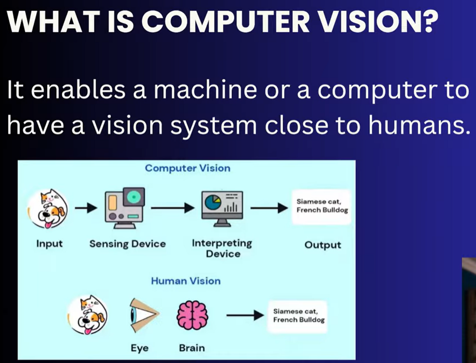
For image processing

opencv
pillow

Core Tasks in Computer Vision

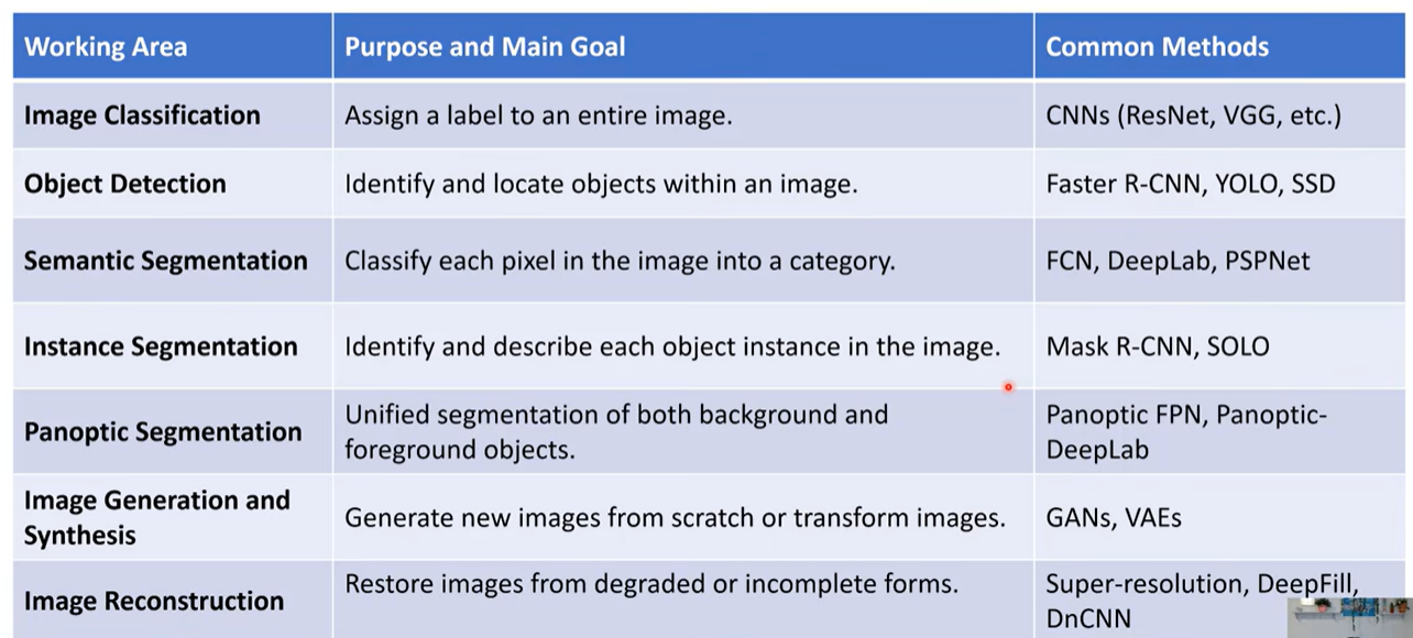
Image Classification: Answering the question: “What is in this image overall?” (e.g., Is this a picture of a human face or an animal?).
Object Detection: Finding where objects are located and putting a boundary around them. (e.g., Your Roboflow model drawing a box around a person’s hand or face).
Face / Pattern Recognition: Identifying specific, unique characteristics within a class. (e.g., Distinguishing your face from a stranger’s face).

Real-World Examples

Self-Driving Cars: Tesla or Waymo vehicles use cameras to “see” lane lines, pedestrians, and traffic lights.
Facial Recognition: Unlocking your iPhone with FaceID.
Healthcare: AI analyzing X-rays, MRIs, and CT scans to find tumors or fractures faster than human eyes.
Social Media: Instagram or Snapchat filters tracking your face in real-time to overlay 3D graphics.
Augmentation like facebook augmentated glass

some challenges for computer vision

Data aquesition
Hardware requirement like tpu GPU, A100
proper knowledeg for this domanin

How to human see any object detection

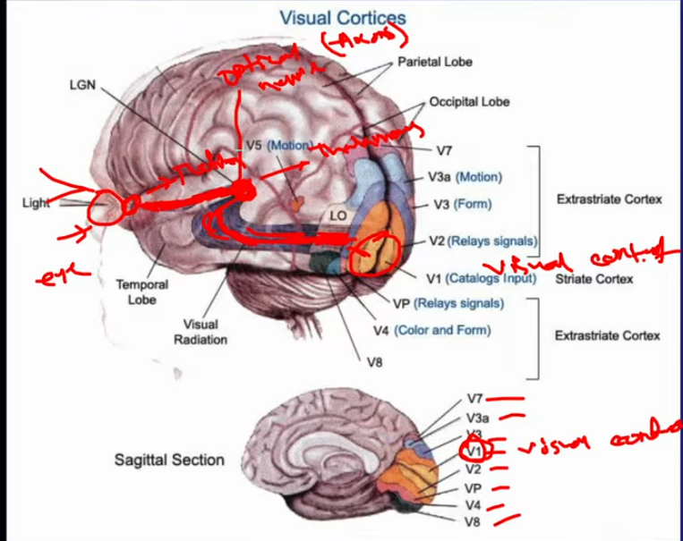
Hubel and Wiesel Cat Experiment

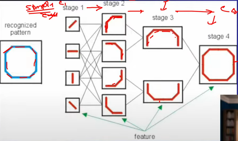
https://www.youtube.com/watch?v=IOHayh06LJ4

Another expriment

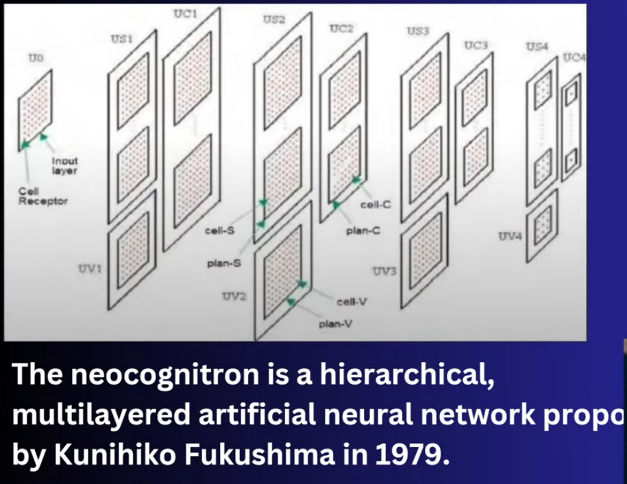
Yanlikan Model

is the father of computer vision and is the now scientis of faceboook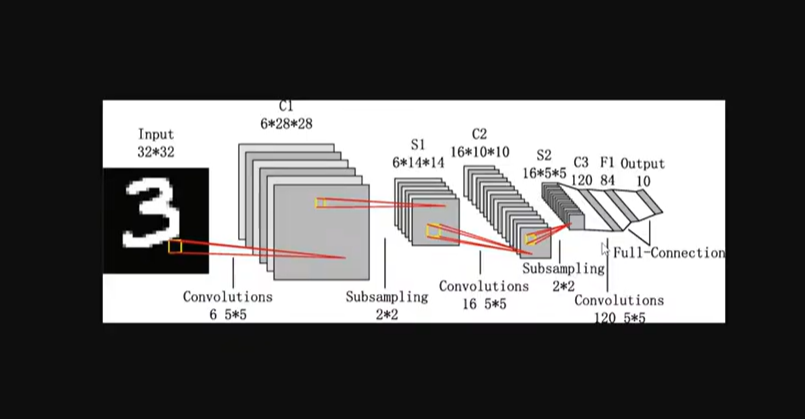

http://yann.lecun.com/exdb/publis/pdf/lecun-01a.pdf

from tensorflow.keras.models import Sequential
from tensorflow.keras.layers import Input, Conv2D, AveragePooling2D, Flatten, Dense

# Create the second model
model2 = Sequential()

# Explicit Input layer (takes 32x32 grayscale images)
model2.add(Input(shape=(32, 32, 1)))

# First Stage: Conv -> AvgPool
model2.add(Conv2D(6, kernel_size=(5, 5), padding='valid', activation='tanh'))
model2.add(AveragePooling2D(pool_size=(2, 2), strides=2, padding='valid'))

# Second Stage: Conv -> AvgPool
model2.add(Conv2D(16, kernel_size=(5, 5), padding='valid', activation='tanh'))
model2.add(AveragePooling2D(pool_size=(2, 2), strides=2, padding='valid'))

# Dense Classification Layers
model2.add(Flatten())
model2.add(Dense(120, activation='tanh'))
model2.add(Dense(84, activation='tanh'))
model2.add(Dense(10, activation='softmax'))

# Print structure details
model2.summary()

Alexnet

import tensorflow as tf
from tensorflow.keras.models import Sequential
from tensorflow.keras.layers import Input, Conv2D, Activation, MaxPooling2D, BatchNormalization, Flatten, Dense, Dropout

# Initialize the Sequential model
alexnet_model = Sequential()

# -------------------------------------------------------------------------
# INPUT LAYER
# -------------------------------------------------------------------------
# Explicit Input layer for 224x224 RGB images (Modern Keras 3+ syntax)
alexnet_model.add(Input(shape=(224, 224, 3)))

# -------------------------------------------------------------------------
# STAGE 1: Conv -> ReLU -> MaxPool -> BatchNormalization
# -------------------------------------------------------------------------
alexnet_model.add(Conv2D(filters=96, kernel_size=(11, 11), strides=(4, 4), padding='valid'))
alexnet_model.add(Activation('relu'))
alexnet_model.add(MaxPooling2D(pool_size=(3, 3), strides=(2, 2), padding='valid'))
alexnet_model.add(BatchNormalization())

# -------------------------------------------------------------------------
# STAGE 2: Conv -> ReLU -> MaxPool -> BatchNormalization
# -------------------------------------------------------------------------
# Note: Reducing kernel size to 5x5; using padding='same' to preserve size
alexnet_model.add(Conv2D(filters=256, kernel_size=(5, 5), strides=(1, 1), padding='same'))
alexnet_model.add(Activation('relu'))
alexnet_model.add(MaxPooling2D(pool_size=(3, 3), strides=(2, 2), padding='valid'))
alexnet_model.add(BatchNormalization())

# -------------------------------------------------------------------------
# STAGES 3, 4, 5: Three Consecutive Conv Layers -> MaxPool
# -------------------------------------------------------------------------
# 3rd Conv Layer
alexnet_model.add(Conv2D(filters=384, kernel_size=(3, 3), strides=(1, 1), padding='same'))
alexnet_model.add(Activation('relu'))

# 4th Conv Layer
alexnet_model.add(Conv2D(filters=384, kernel_size=(3, 3), strides=(1, 1), padding='same'))
alexnet_model.add(Activation('relu'))

# 5th Conv Layer
alexnet_model.add(Conv2D(filters=256, kernel_size=(3, 3), strides=(1, 1), padding='same'))
alexnet_model.add(Activation('relu'))
# Max Pooling downsamples after the 3 consecutive conv blocks
alexnet_model.add(MaxPooling2D(pool_size=(3, 3), strides=(2, 2), padding='valid'))

# -------------------------------------------------------------------------
# CLASSIFICATION HEAD: Flatten -> Dense -> Dropout -> Dense -> Dropout -> Output
# -------------------------------------------------------------------------
alexnet_model.add(Flatten())

# 1st Fully Connected Layer
alexnet_model.add(Dense(4096))
alexnet_model.add(Activation('relu'))
alexnet_model.add(Dropout(0.5))  # Drop 50% of units to prevent overfitting

# 2nd Fully Connected Layer
alexnet_model.add(Dense(4096))
alexnet_model.add(Activation('relu'))
alexnet_model.add(Dropout(0.5))

# Final Output Layer (10 classes for datasets like ImageNet subsets/custom targets)
# Change '10' to '1000' if you are trying to replicate original ImageNet classification
alexnet_model.add(Dense(10))
alexnet_model.add(Activation('softmax'))

# -------------------------------------------------------------------------
# PRINT SUMMARY
# -------------------------------------------------------------------------
alexnet_model.summary()

What is Image Segmentation?

Image segmentation is the process of partitioning a digital image into multiple segments (sets of pixels, also known as image objects) to change the representation of an image into something that is more meaningful and easier to analyze.

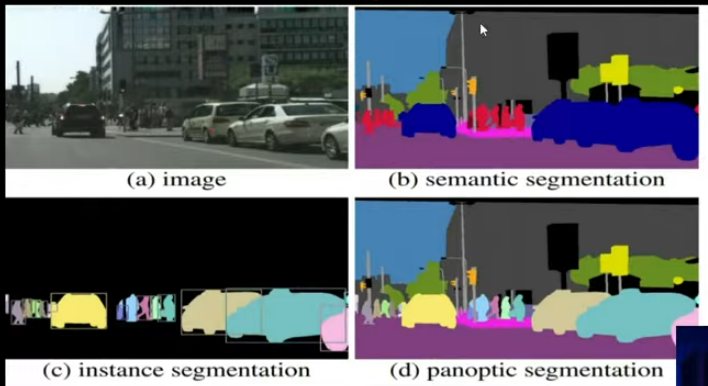
annotation

often called data labeling is the process of labeling your data so the AI can learn from it.

What is an Epoch?

In machine learning and deep learning, an epoch (pronounced “ep-uk” or “ee-pock”) represents one complete pass of entire dataset through the neural network.

what is image

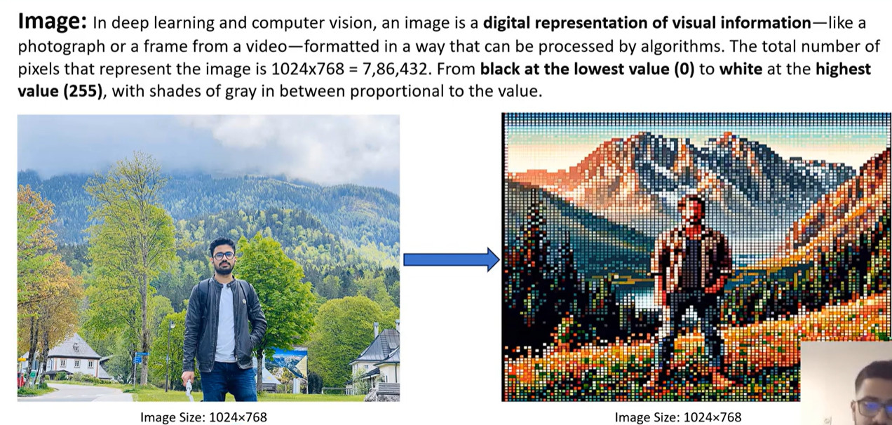
what is pixel

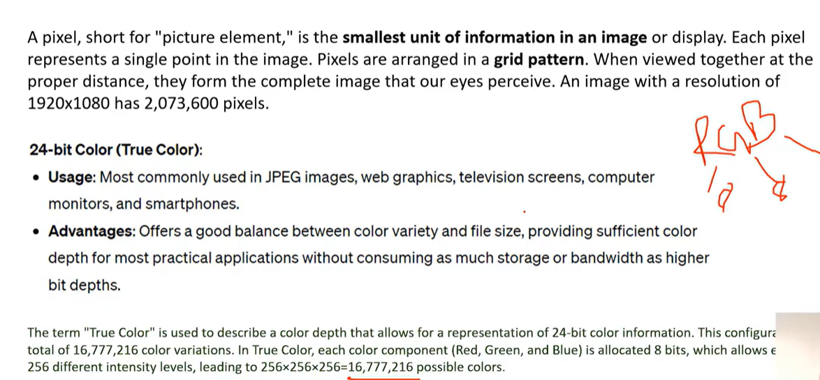
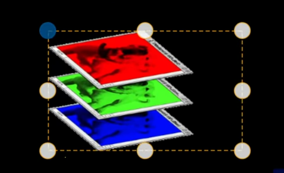
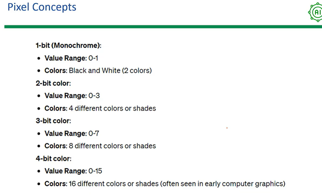
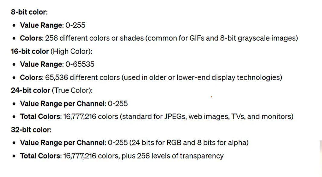
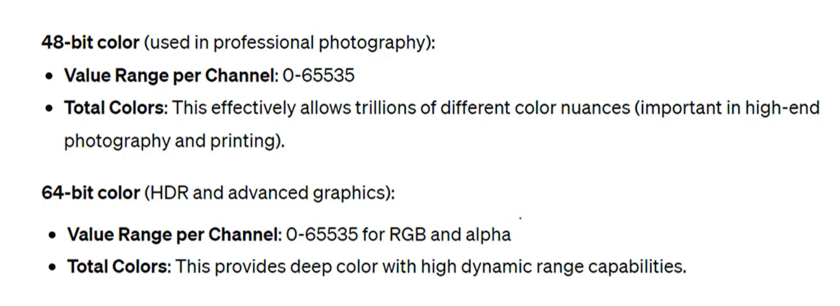
8-bit Grayscale:
These images contain only shades of gray, meaning that each pixel carries information only about intensity of loght or luminance, without any color data.
The values range from 0 (black) to 255 (white), providing a total of 256 different shades of gray.

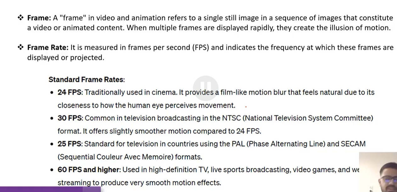
what is video

what is chanel in CNN

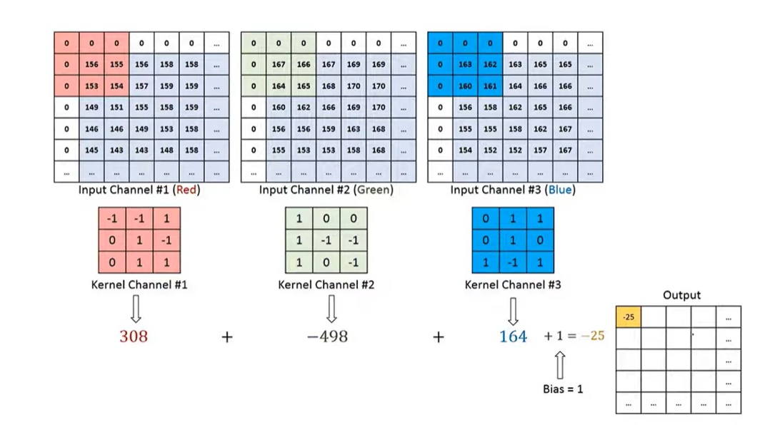
RGB/Color Image: If you provide a colored image, the input layer will read 3 channels (Red, Green, and Blue). Grayscale Image: If you provide a black-and-white image, the input layer will read 1 channel (Luminance/Intensity only).

what is the pooling

what is the flatten

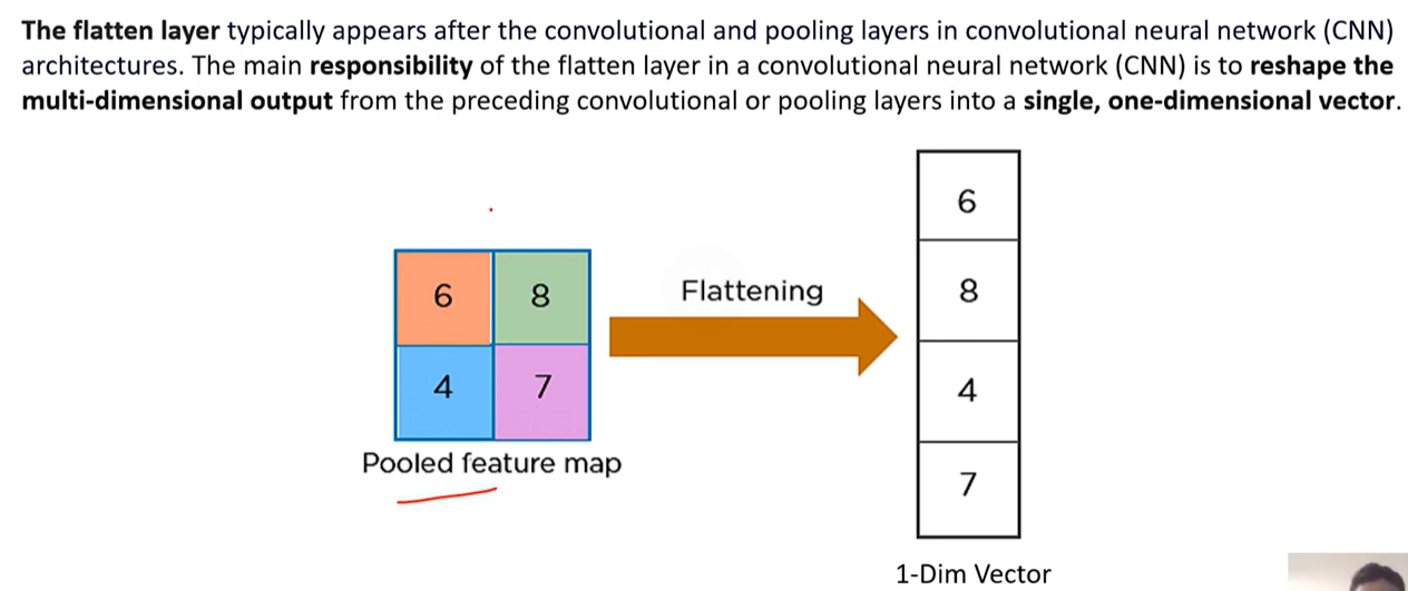
The architecture of CNN

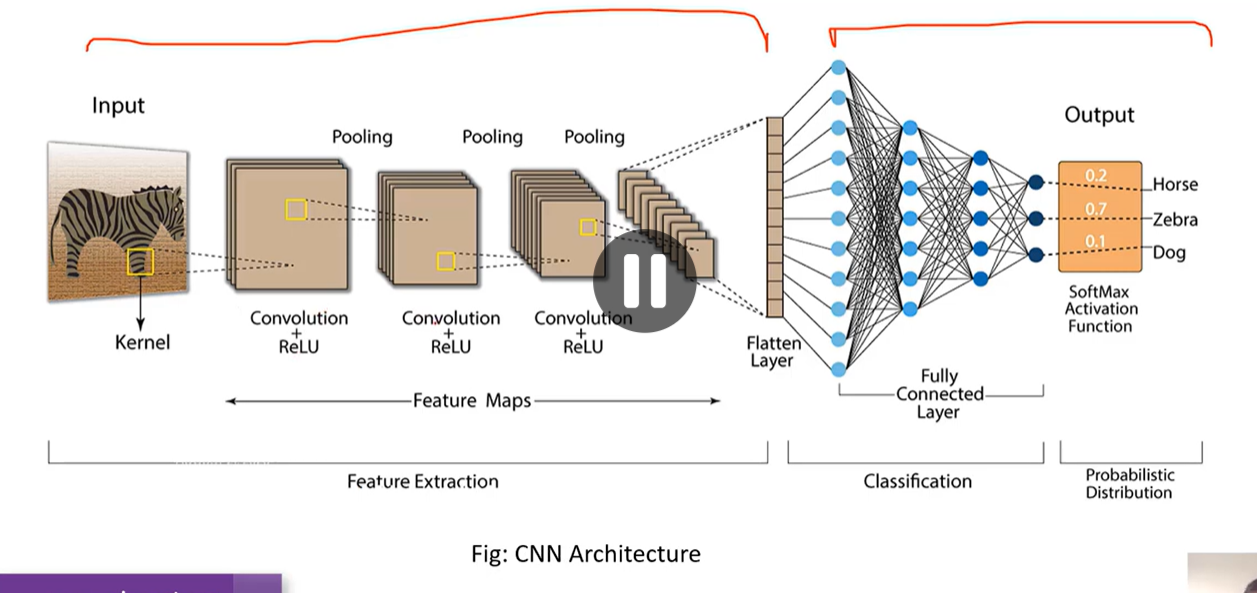
CNN Architecture Breakdown

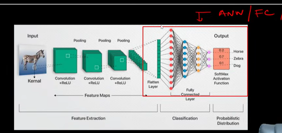
This diagram illustrates the complete, end-to-end workflow of a Convolutional Neural Network (CNN). It outlines how a raw input image passes through multiple mathematical layers to produce a final classification prediction.

The architecture is divided into three major phases at the bottom of the slide:

Feature Extraction
Classification
Probabilistic Distribution

Phase 1: Feature Extraction

This phase is responsible for automatically analyzing the image to detect distinct visual structures, patterns, and boundaries.

Input: The network receives a colorful image of a Zebra. This image contains three structural color layers or channels (Red, Green, Blue). In your specific project context, this input represents the live image of an individual or an intruder captured via webcam.
Kernel (Filter): Indicated by the small yellow bounding box sliding across the zebra’s leg, the kernel is a small matrix that acts as a scanner to detect localized structural patterns like vertical stripes, edges, and textures.
Convolution + ReLU: As the kernel slides across the image, it calculates mathematical multiplications to produce Feature Maps. Instantly, the ReLU (Rectified Linear Unit) activation function replaces any negative pixel values with zero (0), filtering out irrelevant background noise and enabling the network to learn non-linear properties.
Pooling: The feature maps then pass through a pooling layer (typically Max Pooling). This layer reduces the spatial dimensions (width and height) of the maps by keeping only the maximum value within a pixel window, minimizing computational load while retaining vital details.

Key Presentation Note: As shown in the diagram, this combined block of Convolution + ReLU and Pooling is repeated three times in succession. Repeating these layers allows the network to extract hierarchical features—moving from simple lines and edges in the first block to complex facial structures (like distance between eyes, nose width, and jawlines) in the deeper blocks.

Phase 2: Classification

Once the distinct features have been successfully isolated and extracted, the network transitions into its decision-making phase.

Flatten Layer: The output from the final pooling layer is a three-dimensional ($3D$) matrix. The Flatten Layer collapses this multi-dimensional array into a single, long one-dimensional ($1D$) numerical vector. This is visually represented by the tall vertical brown block.
Fully-Connected Layer (Dense Layer): This long vector is fed directly into a dense network of connected nodes, represented by the blue dots. In this layer, every single neuron connects to every neuron in the preceding and succeeding layers. This layer performs high-level reasoning, determining which combination of extracted features correlates with a specific target category.

Phase 3: Probabilistic Distribution

This is the final terminal of the architecture where raw network outputs are translated into human-readable predictions.

SoftMax Activation Function: The final fully-connected layer produces raw numerical scores for each category. The SoftMax function processes these scores, squeezing them into fractions that represent clear percentages. The sum of all output probabilities equals precisely $1.0$ (or $100%$).
Output: In this example, the architecture evaluates three distinct target classes:
Horse: $0.2$ ($20%$)
Zebra: $0.7$ ($70%$)
Dog: $0.1$ ($10%$)
Final Decision: Because the category Zebra holds the highest probability ($0.7$), the system triggers the bounding box labeled “Zebra”.

For your final face recognition application, the output nodes Horse, Zebra, and Dog will be replaced by your designated database target names: Abu Bakar, Enamul, and Uddoy.

Transfer Learning

is a machine learning technique where a model developed for one task is reused as the starting point for a model on a second, related task.it’s alter name is fine tuning

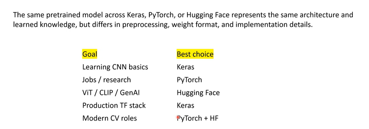
A Simple Machine Learning Example

Imagine you want to build an AI model that can detect rare skin diseases from medical images, but you only have 100 photos of these diseases.

Approach 1: Traditional Learning (Starting from Scratch)

If you train a deep learning model completely from scratch using only those 100 photos, the model will perform very poorly. Deep learning models need hundreds of thousands of images to understand basic visual concepts like shapes, edges, colors, and textures. With so little data, your model will get confused.

Approach 2: Transfer Learning (The Smart Way)

Instead of starting from scratch, you take a Pre-trained Model (like Google’s Inception or ResNet). This model was previously trained on millions of everyday images (cats, dogs, cars, trees, etc.).

Even though this Google model has never seen a skin disease before, it is already an expert at recognizing shapes, edges, patterns, and lighting.

To use Transfer Learning, you:

Take this pre-trained model.
Keep all its basic visual knowledge intact.
Show it your 100 skin disease photos to “fine-tune” its final layers so it learns to apply its shape-recognition skills specifically to medical marks.

The Result: Because the model already knew how to see, it only had to learn what to look for. You get a highly accurate medical model in a few minutes using very little data and computing power.

SOME MODEL

ANN is used to tabular data (This is the foungdation of CNN)

It happend matrix multiplication

CNN is used to image and visualized data (computer vision)

It happend convolution

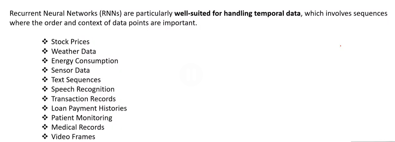
RNN is used for text and audio(Natural language processing)

Vision Transformer (ViT)

is a deep learning architecture that adapts the Transformer model (originally designed for natural language processing) to computer vision tasks.

In 2020, Google introduced a groundbreaking idea: What if we apply this powerful text-based technology directly to images? From that innovation, ViT (Vision Transformer) was born. It processes images by applying the Self-Attention mechanism directly across the visual data, completely bypassing the need for traditional Convolutional Neural Networks (CNNs).

CNN vs. ViT: Key Differences (Based on the Screenshot)

The screenshot perfectly highlights how the inner workings of CNNs and ViTs compare:

1. CNNs (Convolutional Neural Networks)

Use Convolutions: CNNs scan an image using small filters or kernels that slide over the pixels step-by-step.
Learn Local Patterns First: They focus on tiny, local features first—like a specific edge, corner, or texture. They only perceive the broader picture in the deeper layers.
Need Inductive Biases: CNNs rely on built-in assumptions (biases) like locality (pixels close to each other are highly related) and translation invariance (an object is the same regardless of where it appears in the image).

2. ViT (Vision Transformer)

Uses Self-Attention: It completely ditches convolutional kernels. Instead, it uses Self-Attention to calculate how every single patch relates to every other patch in the image simultaneously.
Global Relationships from the Start: ViT captures the entire global context right from the very first layer. It can instantly connect a pixel in the top-left corner with a pixel in the bottom-right corner.
Scales Better with Large Data: While CNNs might plateau, ViT scales incredibly well. When trained on massive, large-scale datasets, it significantly outperforms traditional CNN architectures in accuracy and efficiency.

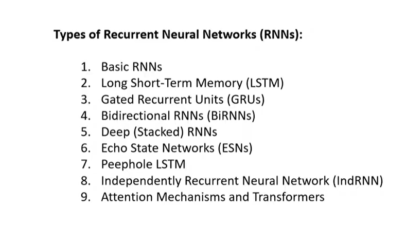
what is RNN

https://www.youtube.com/watch?v=MLrbMHZwuH4&list=PLKdU0fuY4OFdFUCFcUp-7VD4bLXr50hgb&index=39

Yolov5 model

What is PyTorch?

PyTorch is a powerful, open-source machine learning and deep learning framework developed primarily by Meta’s (formerly Facebook) AI Research lab.If you think of YOLOv5 as a high-performance sports car, PyTorch is the factory and the set of tools used to build its engine. It provides developers with the mathematical building blocks they need to create, train, and run Artificial Intelligence (AI) models.